
The Knowledge of Designing and Building Advanced Mobile Robots
A Practical Technical Guide to Mobile Robotics
Pouya Mansournia
Preface to the Global Edition
↑ Table of ContentsThe original Persian edition of this book was published in Iran in 2014 by Simaye Danesh. That earlier edition introduced a practical perspective on designing and building advanced mobile robots for readers interested in robotics, including mechanical and electronic foundations, computer programming, practical projects, component sourcing, and participation in international robotics competitions.
This 2026 global edition is an English, updated, and modernized edition of that earlier work. It is prepared as a technical, academic, and internationally readable guide to the design and construction of advanced mobile robots. It preserves the practical spirit of the original Persian edition while strengthening the engineering explanations, modernizing the computing and software chapters, and clarifying the formulas that connect design decisions to physical behavior.
A mobile robot is not a pile of parts. It is a complete engineered system in which mechanical structure, traction, power transmission, embedded control, sensing, feedback control, autonomy software, artificial intelligence, testing, and safety influence one another. A good chassis can be ruined by poor wiring; a powerful motor can be wasted by weak traction; a beautiful SLAM map can be useless if odometry and coordinate frames are not calibrated.
The intended reader is an intermediate-to-advanced student, engineer, or robotics team member who wants to build real machines rather than only read about them. The tone is deliberately practical: every concept should eventually help the reader choose a part, compute a value, draw a mechanism, write a controller, interpret a sensor, debug a failure, or defend a design decision.
The guiding philosophy of this edition is simple: explain the idea at a level a careful beginner can follow, then state the engineering consequences with enough rigor for university and laboratory work. A reader should finish the book not merely knowing names of components, but understanding why a robot behaves the way it does.
Acknowledgments
↑ Table of ContentsThe author thanks the teachers, engineers, colleagues, friends, and family members whose guidance, questions, and encouragement shaped this work. Their influence remains present in the practical orientation of the book.
How to Use This Book
↑ Table of Contents- Read the mechanical chapters before choosing motors; a powerful motor cannot compensate for poor traction, weak structure, or an unstable center of mass.
- Treat every formula as an engineering estimate that needs measured parameters, safety factors, and test validation.
- Use the ESP32 chapter as a compact embedded-control path, and use ROS 2, Nav2, and AI chapters as the higher-level autonomy path.
- When a paragraph explains an old mechanism, read it as design experience: ask what problem the mechanism solves, what failure it creates, and what a modern implementation would change.
- For every subsystem, write three lists in your design notebook: assumptions, measurements, and failure modes. The difference between a hobby prototype and an engineering robot is often the quality of these lists.
A Senior Engineer's Reading Method
↑ Table of ContentsA senior robotics engineer does not memorize the book from front to back. Instead, they use the material as a chain of questions. What mission must the robot perform? What terrain and payload define the mechanical loads? What sensors are needed to observe the world? What controller keeps the robot stable? What computer runs autonomy? What evidence proves the design is safe enough to test?
While reading, convert each chapter into a design decision. The chapter on tracks should end with a track width, belt type, tensioning method, and service plan. The electronics chapter should end with a power tree, protection plan, grounding strategy, and connector list. The software chapter should end with node boundaries, message definitions, watchdog behavior, and logged test data.
Foundations of Mobile Robotics
↑ Table of Contents
Introduction
History
What Is a Robot?
The first generation of robots was built around 1970. These were stationary robots with no programming capability, built from electronic and mechanical devices with no sensors of any kind. About ten years later, a second generation of robots was designed and built - these had both sensors and programmability. A third generation of robots appeared around 1990, featuring capabilities such as being stationary or mobile, independence and autonomy, and speech recognition. Finally, the latest generation of robots, still in the research-and-development phase today, deals with topics such as artificial intelligence, self-replication, and operating at the nanoscale. Further details of this progression are given below:
1920: Karel Čapek, the Czechoslovak playwright, introduces the word "robot" in his play R.U.R. (Rossum's Universal Robots); the word "robota" in Czech means "tedious labor."
1942: In his story Runaround, Isaac Asimov set out the Three Laws of Robotics:
A robot may not harm human beings.
A robot must obey the orders given to it by a human, except where certain orders conflict with earlier ones.
As long as self-preservation does not conflict with the first two laws, a robot must protect its own existence.
1946: The rise of the computer - widespread use of magnetic tape recording, construction of the first computer at MIT, and the first problem solved by the first digital computer.
1951: In France, Raymond Goertz designed the first remotely operated articulated arm for use in nuclear missions;
The design was based, overall, on mechanical couplings between the primary and secondary arms (using pulleys and spring-loaded cables).
1954: George Devol designs the first programmable robot; the automation era begins...
1959: The Artificial Intelligence Laboratory at MIT is founded by John McCarthy and Marvin Minsky.
1962: The first industrial arms are put into use by General Motors in the United States.
1963: The Artificial Intelligence Laboratory is founded at Stanford University.
1967: The first robot arrives in Japan.
1968: Japan acquires the license to build a hydraulic robot design from the American company Unimation and begins production in Japan.
1968: A mobile robot with machine vision is built, controlled by a computer the size of a room.
1970: A standard arm is designed by Professor Victor Scheinman at Stanford University in the United States.
1973: The first minicomputer for controlling industrial robots is built (designed by Richard Hohn).
1976: The Viking 1 and 2 space probes are used.
1978: Universal programmable assembly machines (PUMA) are developed.
1993: Sensor technology emerges.
1994: The CMU Robotics Institute builds a six-legged walking robot to explore and sample volcanic gases at Mount Spurr in Alaska.
1995: Surgery-related robots are built and put into use.
1997: NASA builds the Sojourner rover to traverse the surface of Mars and send results from the planet back to Earth.
2000: Honda builds a humanoid robot.
2000: Sony builds a humanoid robot.
2001: Sony's second robotics product, known as Sony's robotic dogs (AIBO).
The chart below shows the evolution of robotics in several major industrial countries.
The Meaning of the Word "Robot"
The word "robot" is derived from "robota," meaning labor, and "robotnik," meaning worker.
Definition of a Robot
A robot is an automatic device capable of performing tasks normally attributed to humans.
Robotics Institute of America
A robot (industrial robot) is a reprogrammable, multi-function manipulator designed to move tools, parts, materials, or specialized devices through a variety of programmed motions, in order to perform a range of tasks.
General Overview
Based on the points above, a robot is a programmable machine that imitates the behavior and appearance of an intelligent being (usually a human), and this transformation - turning a machine into a robot - requires meeting the following conditions:
- Sensing and Perception
which includes gathering information from the environment - in other words, receiving information from the surroundings
- Performing a Variety of Tasks
- Locomotion
The ability to perform tasks a human would normally do by hand (manipulation)
- Reprogrammability
A robot must be able to perform different tasks through reprogramming.
- Autonomy or Interaction with Humans
Given the characteristics described above for a robot, several different types of robots can be identified, as follows:
Rescue Robots
When a natural disaster strikes, time is the single most important factor determining the chances of rescuing those affected, and the probability of survival decreases exponentially as time passes. In such critical conditions, cutting search time short means saving more lives, making it a matter of paramount importance. For centuries, rescue dogs have been the most common method for quickly locating victims buried under rubble.
In practice, however, this method has failed to prove fully effective, because the dogs' keen sense of smell - the very reason they're used in rescue operations - keeps them from staying at the scene once the bodies buried under the rubble begin to decompose. Today, new technologies give special disaster-response teams effective tools that, combined with traditional methods, achieve greater efficiency. The idea of using robots in search-and-rescue operations was first proposed in the early 1980s, but no practical effort was made in this area until 1995. In 1995, following the Oklahoma City bombing that killed 168 people, a University of Colorado professor, Dr. Robin Murphy, together with John Blitch of the U.S. Army, began studying the use of robots in search-and-rescue operations. This research led to the definition of a project called the Tactical Mobile Robot project within the Defense Advanced Research Projects Agency (DARPA), affiliated with the U.S. military. In the most significant real-world application of rescue robots - the September 11 attacks - John Blitch, of the National Institute for Urban Search and Rescue, assembled a team of rescue robots from various manufacturers of military robots, such as Foster-Miller, iRobot, and SPAWAR, and used them to help locate victims. The main tasks performed by robots in this incident included:
- Searching for victims
- Finding the fastest route through the rubble to reach a victim
- Technical inspection of the building
- Identifying dangerous or suspicious objects
- Providing information about environmental conditions
- Going to places no living being could reach
Robot Applications Across the Four Environments
One of the most fundamental applications of robots is deployment in places where working conditions are mostly hazardous, difficult, or highly repetitive and monotonous for humans. These environments fall into four general categories:
- Hazardous Environments
- Places where there is a risk of gas poisoning, fire, chemical exposure, physical injury, or some other threat to human life.
- Contaminated Environments
- Places affected by various forms of pollution - noise, chemical, radiation/wave, and so on.
- Monotonous and Tedious Environments
All production work where the manufacturing process involves highly repetitive, tedious steps.
- Harsh and Difficult Working Environments
Work environments that are extremely hot or cold
The Four Core Tasks of a Robot
Another reason for deploying robots is to handle special tasks that humans generally cannot manage, described as follows:
- Automation
- This is the advantage gained in a factory or production workshop by deploying various types of robots, which improves and increases output.
- Augmentation
- Increasing production speed is also made possible through the use of robots.
- Assistance
- Robots are sometimes used to help and assist humans in performing certain tasks.
- Autonomy
- This capability is built into a robot for a specific application (particularly rescue robots or military robots) so it can respond to environmental stimuli - in effect giving the robot a degree of perception and decision-making power under certain conditions and situations.
The other reasons for deploying robots are as follows:
- Improved Production Quality
- Extremely high precision (down to a thousandth of a millimeter)
- Repeatability, which results in consistent production
- Increased Efficiency
- Continuous operation without fatigue
- No need for rest breaks or time off
- Increased Safety
- Operation in hazard-free environments
- No need for environmental facilities such as air conditioning, noise protection, etc.
- Reduced Costs
Robot Challenges
Of course, there are challenges too - like any other machine, a robot can break or fail for any number of reasons. They are also powerful machines that let us control specific tasks. Fortunately, robot failures are quite rare, since robotic systems are designed with numerous safety features that limit the damage they can cause.
Review of Locomotion Mechanisms in Mobile-Base Robots
Simple Track (Belt) System
This robot looks similar to a tank, and it moves like a tank, using tracks. The track stays in place and is driven by a wheel called a pulley. This robot is very well suited to climbing stairs, crossing rubble, and moving through mud. In many rough-terrain conditions, only a tracked robot can do the job. Building this robot exposes the builder to a variety of mechanical challenges - power-transmission systems, track design, track-tensioning systems, and the like - and sometimes forces you into risky territory.
If you're building this robot for very rough terrain, it's best to keep its underside well clear of the ground so obstacles don't get caught underneath. It's also better to use wider tracks for such environments. In more ordinary environments, the robot's ground clearance can be set lower. As ground clearance increases, so does the robot's overall height and, consequently, the height of its center of mass - which in turn makes the robot more prone to tipping over. To keep the robot stable under such conditions, the bottom of the robot should be made heavier to lower the center of mass. This can be done by building the robot's wheels from heavier materials. It's likewise better to build the upper parts of the robot from lightweight materials and structures. When climbing a stair, the length of track in contact with the ground needs to be more than twice the distance between two step edges. It also helps to add lugs on the track so it grips the step edge and climbs more smoothly. If the robot's mission is indoors, its width should be set about ten centimeters narrower than the building's doorways; if the mission is outdoors, it's better to make the robot as wide as possible so that turning happens more smoothly and easily. This increases stability and reduces the chance of tipping over. If the robot needs to move fast and make quick maneuvers, narrower tracks work better. On each side of the robot there is a wheel that receives drive power from the motor and transfers it to the track. The wheels providing drive power can sit at the rear, at the front, or with one at the front on one side and one at the rear on the other. Some robots are essentially four- or six-wheeled, but have a track mounted on them in a process similar to snowmobiles, which ultimately turns the robot into one with a simple track mechanism.
Tracked Robot with Two Arms on One Side
In this mechanism, one side of the robot has two arms, each fitted with a track. When needed, the arm can open outward or close in and tuck alongside the robot. The robot's arms are generally linked together so their rotation is exactly synchronized. This mechanism performs very well in indoor environments, which is why countless examples of it have been built in recent years for military, rescue, and research purposes. For a tracked robot to be able to climb stairs, its length must exceed twice the distance between two step edges. If the robot is too long, its maneuverability suffers. This design has the advantage that, with the arms open, it gains the capabilities of a long robot, while with the arms closed, the robot becomes shorter and gains the advantages of a shorter robot. At the start of a climb, the arms must be open at an angle so the robot can pull itself up over the step edge; after that, the arms must swing fully open to horizontal so the robot can move across the steps.
In these robots, two motors drive the tracks on the robot's left and right sides, while a third motor drives the arms. The arms can rotate around their axis without limit. This robot can be designed and built using countless different mechanisms - for example, the drive motors can transmit power to a pulley. Below is a description of the mechanism used to build this robot, produced and tested by the authors, whose design and construction was achievable without complex manufacturing techniques.
In the proposed mechanism, drive power from the motors is transmitted to the rear pulley, and the rear pulley transmits that power to the front pulley via a belt. At the front there are two pulleys connected to each other - one belonging to the robot body and the other to the arm. Drive power passes to the arm through these two connected pulleys, driving the track on the arm.
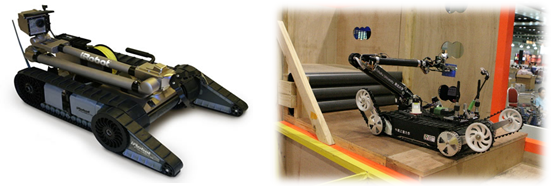
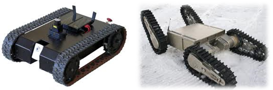
Figure 1-4. Left: an example of the robot with its arm open. Right: a robot built specifically for irregular warfare that is easy to carry.
It's recommended that the arm be no shorter than half the robot's total length, since a shorter arm won't deliver the performance needed. The diameter of the pulley at the arm tip isn't a critical factor and can be any size - though weight still needs attention, since if it's too heavy, the robot's center of mass shifts forward when the arm opens.
Many designers, at the start of a design-and-build project, try to build a robot that can also move easily on its back if it flips over. In reality, this type of robot doesn't flip over easily, and pursuing a design meant to work both right-side-up and upside-down limits you unnecessarily - the drawbacks far outweigh the benefits. Because of this robot's structure, its ground clearance is low, so it runs into trouble moving through very harsh terrain such as rubble. That said, the rubble fields in rescue-robot competition arenas are much gentler than real rubble, and this robot can handle them just fine. For indoor missions, this robot is the best option available. The arm's rotation is driven by a motor and a gearbox. A worm gearbox is recommended, since it locks in place when the motor stops, removing the need for electronic motor locks. It's best to use commercially available worm gearboxes. Some teams lose time trying to build their own gearbox, and the rework caused by mistakes ends up costing the team more than a ready-made gearbox would have. Remember that robotics is the art of using modules - wherever a module already exists, you shouldn't be manufacturing the part yourself. The available worm gearbox has a single input, connected to the motor, and two outputs on the left and right through which the arm shafts pass. Use one shaft for both arms and attach an arm to each end. Fix bearings onto the arms and mount pulleys onto the bearings. These robots are generally heavier at the front than the back, which keeps the center of mass from sitting at the robot's midpoint. That, in turn, keeps the robot from rotating cleanly in place - turning becomes awkward and the robot is harder to steer. The robot's design must therefore account for where the center of mass sits and correct for it. There's a gap between the robot's front and rear pulleys that isn't well suited to mounting most equipment and is, in effect, dead space - a good spot for mounting batteries. Of course, achieving a proper center of mass may require designing the rear of the robot to be heavier, which can be done by moving the batteries toward the back.
In these robots, aside from the main pulleys, there are usually no other idlers. Some builders, however, add one or more idler pulleys in the gap between the front and rear pulleys. Looking at the problem systematically shows that this idler pulley helps the track run properly on large robots and keeps it from coming off. A suspension system is therefore not recommended. If a tracking/suspension capability is needed out of necessity, the system should be designed so it can be locked in place, with its effect removable through a simple action - such as tightening a screw or inserting a pin - whenever needed.
This robot is introduced here. It consists of four sections with similar structure, two of which act as arms. The arms can open and close independently of one another. The two middle sections are heavier than the other two, so the robot's balance isn't disrupted while the arms are opening.
This robot has several exceptional features:
- Because its surface is covered in track, obstacles don't catch on the robot, letting it cross even the harshest terrain.
- With its arms open, the robot can move inside vertical shafts and fixed pipes.
- The robot can fold into a figure-eight shape and move much like a four-wheeled robot.
Two-Tier Track System
This robot is built to pass through narrow shafts and can climb inside vertical channels. It also carries tracks on its top and bottom, and the gap between top and bottom can be adjusted so it grips the shaft properly. At the front, between the upper- and lower-tier tracks, sit arms that, besides supplying part of the drive force, let the robot cross rough terrain properly. A camera and vision equipment are mounted on one of these arms. A good choice of track material for these robots is a timing-belt system covered with a suitable coating, such as friction belting. To adjust the gap between the robot's two tiers, there is a motor and a ball-screw mechanism that controls the spacing of certain chassis parts and, through them, the distance between the two tracks. This robot carries limited onboard electronics, and its drive power is supplied via a cable from outside; communication signals are likewise exchanged between the robot and the outside over a wired link. This robot's chassis is of the pillar type, and the whole chassis-and-parts assembly is very lightweight, since low weight increases the robot's stability inside vertical shafts and prevents damage to the shaft walls. The robot's speed is also very low, since it has to be steered with great precision. It is operator-controlled and has no artificial-intelligence capability.
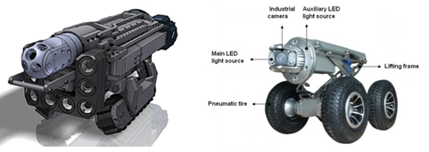
A steel cable is attached to the rear of the robot so it can be pulled back if needed, and to keep the other cables from being pulled taut. Instead of a steel cable, lightweight cables such as Kevlar - which combine low weight with high shear strength - can be used. These are among the highest-quality climbing cables available and come in a range of diameters.
Tracked Robot with Four Arms on Both Sides
This robot moves on tracks, with four arms at its front and rear, each also fitted with a track and its own drive force. It is well suited to indoor operations and can climb stairs and inclined surfaces. In recent years this mechanism has been very popular, and many operational and research robots have been built on this basis. A considerable number of these robots serve as rescue robots and bomb-disposal robots. At the front and rear of this robot sit four tracked arms. The arm tracks are driven and draw their power from the robot's main tracks. The arms can increase or decrease how much of the track surface contacts the ground, which lets the robot adjust its own stability and get over obstacles such as steps. Most designers couple the front and rear arms together in pairs, though some give the arms more freedom, assigning each an independent degree of freedom. Given the sheer volume of mechanical components in this robot and the limited space available for design, most designers choose the first approach.
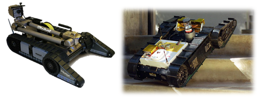
The advantage of this approach is its strong ability to get over indoor obstacles such as ramps and stairs; its limitation is slow movement over natural obstacles such as rubble and rocky terrain. On top of that, the volume and number of mechanical parts in this robot is high, which makes it hard to design, drives up its weight, and - worst of all - leaves very little space for the electronics team to fit in components. Many varieties of this robot have been built, generally falling into four categories, classified by how the main track and the arms are arranged. The four categories are:
Inner Main Track
In this approach, the robot's main tracks are attached to the main chassis, and the arms are mounted farther out than the body and main chassis. Two motors generate the robot's driving force and transmit it to the robot's tracks; the main tracks then pass the power they receive on to the arm tracks. Compared with the other approaches, this one has seen more use and attention. Typically the main track's drive pulley is directly coupled to the arm's base pulley, transferring power from the main track to the arm tracks this way.
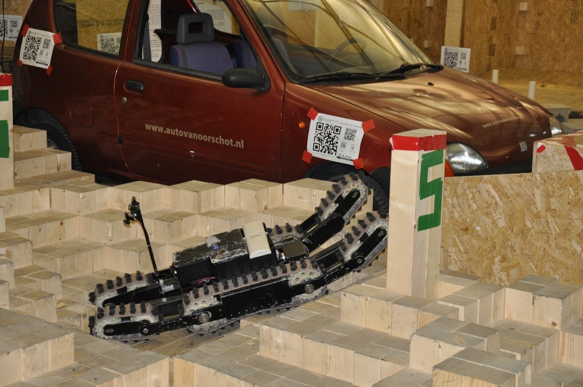
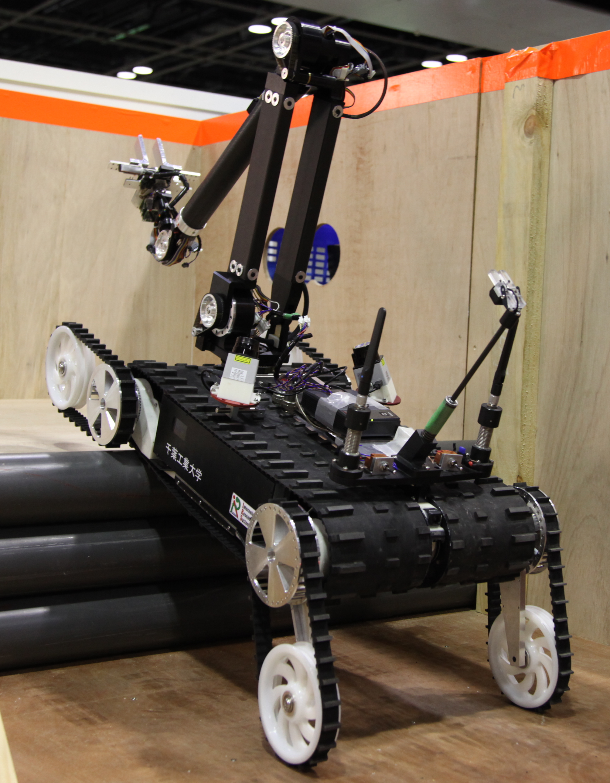
Figure 1-5. An example of a robot based on the inner-main-track approach
Outer Main Track
In this approach, the arms are attached to the robot's body, and the main track sits farther out than the main body.
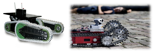
The robot's drive power comes from two motors, each driving one side of the robot. Power from the motor passes to the track of one arm, then from that arm's track to the robot's main track. From there, power passes from the main track on to the other arm's track. Some of these robots are built so the arms on one side can fold inward, tucking into the gap between the main track and the robot body.
Single Track
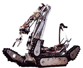
This approach is rarer than the others and less reliable. Here, each side of the robot has one long track that serves as both the main track and the arm track, using fewer mechanical components than the competing approaches. The challenge facing the designer is that this track is difficult to tension - in other words, adjusting how loose or tight it is proves very difficult.
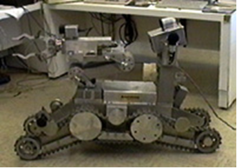
Figure 1-6. An example of a robot built on the single-track approach
Matching Tracks
Each arm of this robot has two narrow parallel tracks, and the main tracks share this same feature. A row of tracks also transmits power from the main tracks to the arm tracks. Designing and building this robot is harder than the other similar types. Each arm consists of two halves - the first connects to the robot, and the second connects to the first. The first half carries a gearbox that, as it rotates, drives the second half to rotate faster.
Four-Arm Tracked Robot
This robot has only four tracked arms and has been widely built for operational uses such as bomb-disposal robots. A considerable number have also been built for research and robotics competitions. When all of the robot's arms are raised, a small, rounded section of each arm rests on the ground, giving the robot behavior similar to a four-wheeled robot. Turning in these robots resembles a bulldozer, achieved by rotating the left and right tracks in opposite directions. Turning this type of robot places destructive forces on the arms, which must be carefully analyzed and neutralized during design. When the robot rests on the tips of its four arms it sits at its greatest height; when the arms are raised so the robot rests on the arm bases, it sits at its lowest. In the first configuration, turning the robot in place is not really attempted, since the forces involved would most likely damage the system. In the rarer of the two configurations, the arms are very long relative to the body, and the arm bases sit very close to one another.
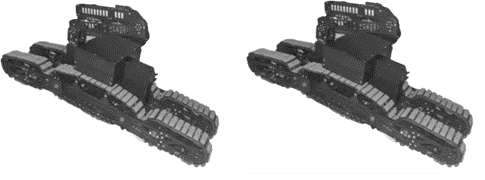
Figure 1-7. The Kafin robot: built by the author, with its motors housed inside the driving arm.
In the second, far more common configuration, the arms are not particularly large in length or volume relative to the main body. In these robots, the drive force on each side comes from a single motor and is transmitted to the two tracks of the arms on that side. In most robots, the front two arms and the rear two arms share a common rotation axis, so the front arms rotate together via one motor and the rear arms rotate together via another. In a few robots, each arm instead rotates via its own independent motor.
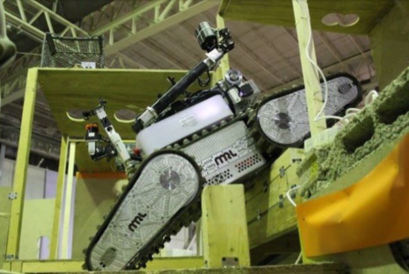
Because of the stress placed on their arms, this type of robot needs to stay lightweight to ease that stress, making a pillar-type chassis the right choice. Some designers, to reduce the effect of arm stress, connect the two ends of the front and rear arms together with a rod. If the arms are small enough, they can rotate completely and without limit without interfering with other components. Most four-arm robots can get over difficult obstacles such as stairs. Laying the arms flat on the ground fully increases the robot's stability and helps it pick up heavy loads off the ground without tipping over. With the arms fully flat on the ground, the robot can climb very steep slopes. This robot's most important and distinctive capability is crossing narrow streams and channels.
Combining a Four-Wheel Robot with a Four-Arm Track System
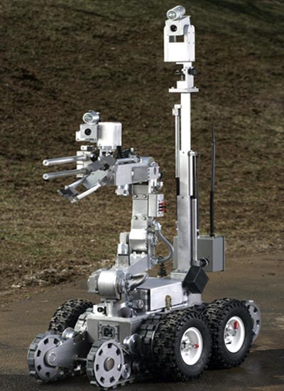
This robot has exactly the same mechanism and structure as the four-arm tracked robots, except that the pulley at the base of each arm is connected to a wheel - usually an inflatable one - which eliminates much of the rough ride otherwise caused by the robot's movement. Because tracks are thin and carry lugs, most tracked robots move with a great deal of bounce and vibration. Adding wheels to four-arm tracked robots brings the advantages of wheeled robots into this design. It also retains the important capability of climbing stairs and crossing channels such as gutters. And when the robot's arms lie fully flat on the ground, its stability increases greatly, letting it pick up heavy loads off the ground without tipping over.
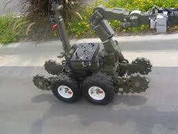
Research prototypes of this robot are limited, but in operational use, many bomb-disposal robots draw on this mechanism. Many of these robots are built so that, when needed, the wheels can be detached by hand using a lever similar to a bicycle quick-release seat clamp, turning the robot back into its original tracked form. This process narrows the robot, making it better suited to indoor missions.
Folding Track System
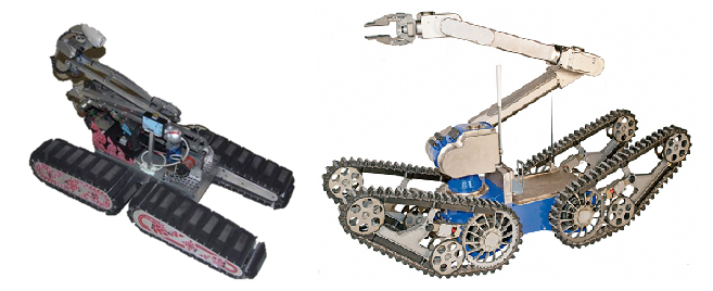
In this system, the robot is built from two sections joined together at one end. At the joint sits a motor and a powerful gearbox that lets the two sections take up different angles relative to one another. These robots are generally built for research purposes. There are three variants of this design, as follows. The most common variant is built from two dissimilar sections: the front section is shorter and narrower than the rear, which supplies the drive power. This robot is built for indoor movement and can overcome obstacles such as stairs; it doesn't perform well on very rough terrain such as rubble, since its underside - which normally sits close to the ground - snags on obstacles. Propulsion comes from two motors, whose power goes directly to the rear pulleys of the rear half. That power travels by track from the rear pulley to the front pulley of the rear half; the front pulleys of the rear half connect to the rear pulley of the front half, so the rear half's propulsive force carries through to the front half. To change the angle between the two sections, the robot uses a motor and gearbox - generally a worm gearbox. The front section must be lighter than the rear so it can lift and pivot away from the ground when needed. It's best to place heavy parts such as batteries and motors in the rear section, with control electronics up front. Because this robot's center of mass sits toward the rear, it can't turn in a balanced way once its front section is resting on the ground, so it's better to keep the front section slightly above ground level during normal travel. Since the tracks, besides driving the robot, also carry drive power through to the front half, most builders use double-sided timing belts or similar timing-belt products as the track. In the rear section every pulley must be a timing pulley; in the front section the rear pulley must be a timing pulley, but the front pulley can be a simple cylindrical roller instead. A second variant consists of two nearly identical robot halves joined together, typically with one or two degrees of freedom between them. This robot can be designed for indoor use or for complex outdoor environments such as forests. Each section has a structure similar to a simple tracked robot, with one or two motors and gearboxes sitting between the sections to create one or two degrees of freedom. If built for indoor operations, the front half should be lighter than the rear half so that, on meeting a stair, it can lift its front half up onto the step. For robots operating outdoors, such as in forests, the underside should stay clear of the ground so it can engage with obstacles.
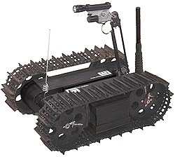
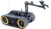
A third, much rarer variant consists of two similar sections, each carrying only a single track positioned between them; this track is very wide and effectively covers almost the entire underside of the robot. These robots suit missions on very slippery ground, such as snow and ice. The two sections have two degrees of freedom relative to each other, and the robot turns much like a wheel loader, articulating in the middle. Some builders mount lightweight parts on both sides so the robot can float on water; its structure lets it glide gently across still water by rotating its tracks. Because the surface is covered by tracks, access to the electronics is somewhat difficult. These robots are built to pass through small passageways and are relatively small; observed examples have mostly served rescue purposes. In this robot, the front pulley shifts out of its normal position and moves to the top of the robot, shortening its length while increasing its height - a trade-off that can be useful depending on the situation. The track is a timing-belt type, coated with a covering such as a wear-resistant belt, with drive power transmitted to it from the rear pulley. The rear pulley is a timing pulley, while the others are simple cylindrical rollers; all pulleys carry flanges so the track can't come off. Drive power comes from two motors, which can connect directly to the rear pulleys. The chassis has three sections: two at the rear (left and right), with the rear pulleys attached at their ends, and one at the front-center, to which the front pulleys attach; the two rear chassis sections connect to the other end of the center section through a bearing. The end of the center chassis connects, via a bearing, to the midpoint of the two rear sections, and a motor and gearbox drive its rotation about that bearing. This way, the front pulleys can sit either at the front of the robot or on top of it. The parts fixed to the two rear chassis sections and the center section are heavy, keeping the robot stable while it changes shape.
Track System with One Wheel on Each Side
On each side of some tracked robots sits a wheel with no drive force of its own. Designers use this layout for two main reasons. First, on some robots the track sits high enough off the ground that the robot struggles to climb stairs. To fix this, a fairly large wheel is mounted at the front of each track, positioned higher than ground level so that the point where it meets a step edge sits below the wheel's center. When the robot reaches a stair, the forward-driving force of the tracks pushes the wheel against the step edge and climbs it. As the robot is pulled upward and continues forward, it engages with the step itself shortly after; because of the wheel's large diameter and height, the front of the robot is lifted high enough that the step edge meets a point below the center of the front pulley, letting the robot settle onto the steps and climb them with ease. This technique is mainly used on larger robots. On some robots the wheel is mounted at the tip of an arm whose angle can change, letting the wheel's height above the ground be adjusted to suit the situation. The left and right arms change angle together, driven by a single motor in sync; it's best if the arm's motor and gearbox are a powerful motor paired with a worm gearbox. That said, since this is my own idea and hasn't been rigorously tested, it may not turn out to be practical.
Quadruped Galloping Mechanism
This is the fastest gait among four-legged animals, called the "gallop" in horseback riding. Animals such as cheetahs use this gait when running at high speed. To describe the method, the stages of one gallop cycle are shown in the table below:
- The front legs are off the ground while the rear legs are on the ground, driving the robot forward.
- The front legs are off the ground and the rear legs are on the ground, driving the robot forward and about to leave the ground themselves.
- Both front and rear legs are off the ground, and the robot moves forward rapidly through the air.
- The front legs are on the ground and the rear legs are off the ground.
- The front legs drive the robot forward while the rear legs stay off the ground.
- The front and rear legs are tucked in, with none touching the ground; in this phase the robot moves forward rapidly through the air.
- The front legs tilt forward and the rear legs touch down, and the robot re-enters the first stage of the running cycle.
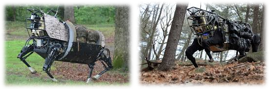
In this gait, the two rear legs don't necessarily touch the ground at exactly the same instant and may differ slightly from each other; the front legs are no exception. On the surface, this method looks like it would create balance problems, and it's tempting to assume the robot would tip over - but that doesn't happen. The reason lies in a matter of mechanics that's difficult to explain and falls outside the scope of this book. For an intuitive sense of it, though, think of a motorcycle's balance at high speed: however the rider shifts around, the vehicle doesn't lose its balance.
Six-Legged Robots
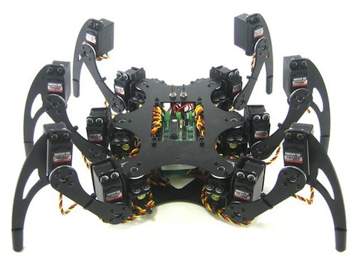
Insects have always been a rich source of inspiration. Their extraordinary locomotion abilities have driven extensive research, and countless robots have been built with three pairs of legs, just like insects. Such robots have been built across an enormous range of sizes, from a few grams up to many times that. Today there are machines used in forestry work that walk easily on six legs, and many robots have also been built to study whether this kind of robot could be used in space.
Studying insects reveals many different walking patterns, but the general method works like this: the insect lifts the front and rear legs on one side together with the middle leg on the other side, and swings them forward. Meanwhile, the legs still on the ground change angle relative to the body, driving it forward. Once the lifted legs have advanced far enough, and the grounded legs have moved the body forward by the same amount, the lifted legs touch down and the previously grounded legs lift off. Adjusting stride length and the speed of this cycle lets you increase walking speed. Turning follows a similar process, except the legs on each side move in opposite directions for forward motion. One mechanism found in insects that has also carried over into robotics has the robot move sideways - left and right - instead of forward and back. Here there's no turning in place, so the insect must fall back on the previous walking method; it's best to combine both methods to improve overall mobility. In this method, the robot first lifts the middle leg on one side along with the front and rear legs on the other side. As it does, the knees of the left and right legs bend in opposite directions, shifting the robot to one side. The lifted legs then come down while the other legs lift off, and the whole sequence repeats. These two walking methods are described here only briefly - the reality involves more detail. The main platform of six-legged robots is built in one of two shapes: usually rectangular, though sometimes round, with round-platform robots turning more easily and precisely. There are seven common approaches to building a six-legged robot: the first five replicate insect movement, while the last two bear little resemblance to how insects actually walk.
In the first method, hydraulic or pneumatic actuators drive the legs - an approach typically used in heavy machinery. These robots generally use linear actuators, with each leg carrying two degrees of freedom. On each side, five identical gears transfer power to one another through a gear train, and the legs connect via a bearing to the front, rear, and middle gears. This robot cannot move sideways.
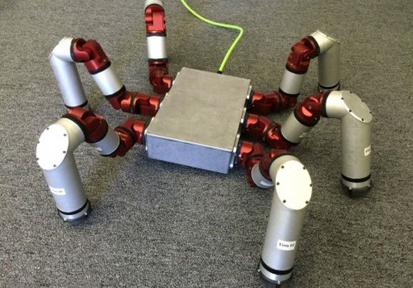
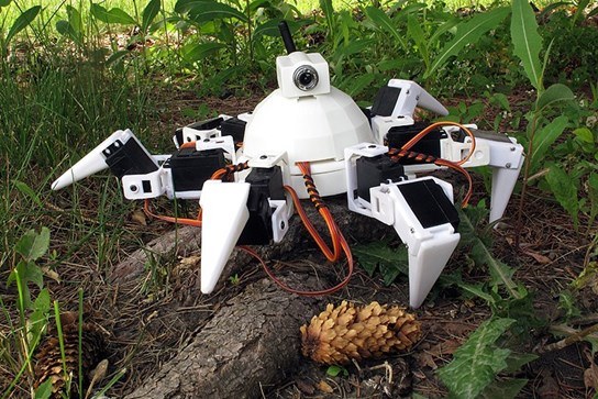
In the fifth method, a clever design lets you build a six-legged robot easily with just two or three linear or rotary actuators. Here, each left leg connects directly to its corresponding right leg - more precisely, each left leg and its right-side match form a single metal strip bent at several points. Each leg pair connects at its midpoint to a rod, with one degree of freedom relative to it, and the front and rear leg pairs are arranged so the whole thing acts like a seesaw: as the left leg swings forward, the right leg swings back. Through this simple rod linkage, when the front-right leg moves forward, the rear-right leg moves forward too - in effect, all four front and rear legs are linked so a single actuator can drive them all. The two middle legs are connected the same seesaw way: as the left one goes down, the right one lifts off the ground. When the middle leg on one side goes down, both legs on that side lift off and the robot rests on that leg's foot, while the legs on the opposite side pull the robot forward. This cycle repeats continuously. The robot has two flaws that keep it from being a real operational design. First, it drifts to one side with every step - slightly left on one step, slightly right on the next - giving it an uneven, lurching gait. Second, it cannot turn. The first flaw simply has to be accepted; fixing the second means altering the structure slightly so the front and rear legs on each side share one actuator while the left and right sides run fully independently - giving the robot three actuators in total. The sixth method, which the author calls the "firefly method," is a rare approach that has drawn little attention. Here, each leg has one degree of freedom relative to the main body and can swing forward or backward, while the main chassis consists of two sections that rotate relative to each other. The stages of one walking cycle for this robot are as follows:
All legs are on the ground, forming a ninety-degree angle with the main body. The rear and middle legs change angle by equal amounts, shifting the center of mass from the middle toward the rear of the robot. The two body sections change angle relative to each other, and the front legs lift up. The front legs change angle relative to the body and swing forward. The angle between the two body sections changes, and the front legs come down onto the ground.
The angle between the two body sections changes and the middle legs lift off the ground. The rear and front legs change angle relative to the body, moving it forward, and the middle legs move forward as well. The front and rear legs keep changing angle to tilt the robot forward, and the angle between the body sections changes so the middle legs come down to the ground, with the front and rear legs now forming roughly a ninety-degree angle with the main body. The front and middle legs change angle, driving the body forward and shifting the center of mass forward too. The angle between the body sections changes so the rear legs lift off the ground. The rear legs' angle relative to the body reaches ninety degrees, and the body sections change angle relative to each other so the rear legs come back down.
Eight-Legged Robots
These robots resemble spiders, one of whose defining traits is having four pairs of legs. Only a handful of robots have been built with four leg pairs so far, mostly for research purposes. Most of what was said about six-legged robots applies here too, and the small differences aren't hard to grasp.
Robot with Six Crescent Wheels
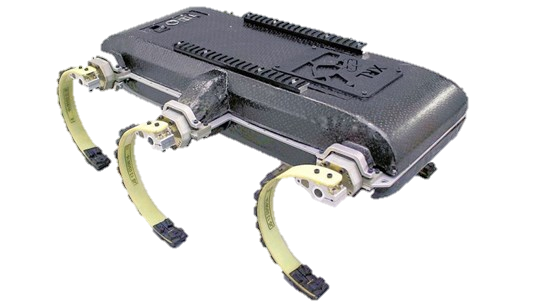
This robot's structure resembles that of six-wheeled robots, except it has no wheels - its axles connect instead to crescent-shaped rods, and the robot moves by rotating these crescents about their axis. It's built mainly for research, though it also has strong potential for operational use. This robot can cross obstacles such as rocky terrain and stairs, and if the water can support it, it can keep moving across the surface. Its movement and steering resemble a six-wheeled robot's: to move forward, the axles connected to the legs all rotate forward together; to turn, the left and right axles rotate in opposite directions.
The wheels - or rather, legs - of this robot are crescent-shaped and springy. Each leg may be made of two segments hinged together with a spring between them, giving the leg its give. This robot generally moves roughly, sending shocks and mechanical vibration through all its components; the springs cut these shocks down significantly and protect the robot from damage. Because the terrain they work in is so demanding, these robots are typically built so that, even flipped over, they keep moving just as before - the robot effectively has two working sides, with no real concept of "top" or "bottom." It has no suspension system, since its violent motion would wreck any suspension's effectiveness anyway; the springy legs make up for this to some extent. There's one motor on each side, and its power reaches the three legs on that side through a transfer system such as a chain. The chassis can be built in various ways, but lightweight, rugged designs such as a pillar-type chassis suit it best.
Motors
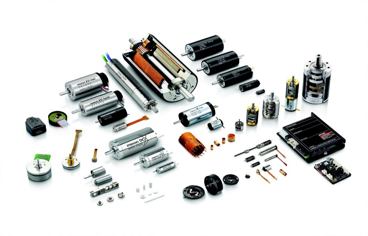
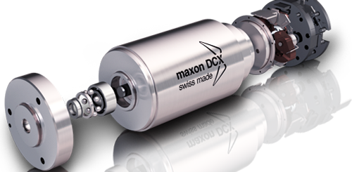
DC motors hold a special place in industry today. Thanks to their high efficiency, broad range of applications, and ease of control, they're used more than any other motor type - qualities that make them especially well suited to countless devices. Starting a DC motor takes nothing more than applying voltage to it; reversing its direction just means reversing the supply current's polarity; and varying the applied voltage lets you control both its torque and its speed. In mobile-base robots, motor torque and speed are two fundamental factors, and when choosing a motor you must always factor in the battery's power capacity as well. One of the best robotics motors is made by the Swiss company Maxon Motor, known for exceptional precision and refinement - though these motors cost somewhat more than Taiwanese or German alternatives.
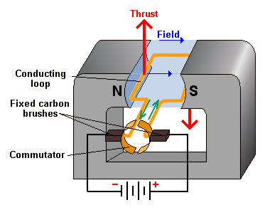
How a DC Motor Works
In a DC motor, a permanent magnet creates a magnetic field, and the rotor spins inside it. The rotor, at the center of the motor, has a number of "poles," each wound with a coil. The coils connect, at the center of the shaft, to a switch known as the "commutator." The brushes connect to the motor's + and - wires (which feed the coils) in such a way that one pole repels the magnetic field while the other attracts it. As the rotor turns, the commutator reverses the direction of the magnetic field, and the presence of multiple poles keeps the rotor's motion going. The brushes feed the motor so that the rotor's magnetic field is always chasing the magnet's field, and this is what drives the motor's rotation. Passing more current through the coils strengthens the magnetic field and spins the motor faster. As the coils move through the stationary magnetic field, they generate a current of their own, with polarity opposite to the current the motor draws from the battery. This current is known as the "back current," or CEMF (counter-electromotive force). What matters about this current is that once the rotor reaches a point where CEMF is present, it draws current to cancel out the load placed on the motor, and the motor settles into a steady state. If there's no load on the motor, this is the point of highest efficiency - though it's also the weakest point in the motor's working range. The strongest point in the motor's working range is where no CEMF is present at all: here, all the current drawn goes toward driving the motor, and the amount of current is proportional to how the motor is moving. When the rotor comes to a complete stop under load, the current at that point is called the "stall current," and the motor delivers its maximum torque in this state. The highest current value (stall current) is also drawn when the motor starts up.
Sizing a DC Motor
Many students shy away from this topic because of its complicated math. If you're interested in robot design done rigorously and scientifically, you need to be able to pull a motor's specifications from its datasheet before buying it. On top of that, once you've worked through this section, you'll be equipped to make selections for other engineering projects as well.
By definition, "torque is the vector force a motor can produce at a given distance from its shaft." Suppose a motor lifts a weight off the ground using a string wound around a pulley of a given radius. If the motor lifts a one-kilogram weight using a pulley with a one-meter radius, the resulting torque is 9.8 newton-meters. Where the metric system isn't used, pound-feet and ounce-inches take the place of these units - though the relationships hold the same across all unit systems. One inch equals 2.54 centimeters, and one meter equals 100 centimeters. It's worth noting that one full revolution equals 2π radians. Mechanical power, in watts, is calculated from the following relationship:
In the relationship above, T is the measured torque in newton-meters, and ω is the angular velocity in radians per second. This formula describes a motor's power at every point in its operating range. Suppose a DC motor runs at maximum power, at half its maximum torque and half its maximum angular velocity. Maximum power can then be calculated from the following relationship:
Where angular velocity is at its maximum, torque is at its minimum, and where torque is at its maximum, angular velocity is zero. Figure 4-1 illustrates this relationship more clearly. Note that as the motor's rotational speed (RPM) increases, torque decreases. At a certain point, power output peaks, and beyond that point power begins to fall. This point is called Pmax.
When selecting motors for use in robots, we're usually looking for the optimum speed and the highest power across the motor's operating range. For most DC motors, this optimal point occurs at about 10% of stall torque, lower than the torque at maximum power. To work out the power a DC motor needs, first determine the power required to move the robot, then, by checking motor specifications, choose a motor whose Pmax exceeds that requirement. Make this choice so that, at the target speed, the motor delivers the required power while drawing the least current possible - a larger motor can help achieve that lower current draw. You clearly need to know the no-load speed and measure the motor's maximum torque (at the point of maximum power); all of these values can be measured fairly simply. If the seller doesn't provide these specifications, you'll have to buy the motor first and measure the values yourself. To calculate Pmax you may need to convert units; before reaching for other reference books, here's how it's done:
For example, 100 RPM equals:
To convert ounce-inches to newton-meters (for T), proceed as follows:
For example, 100 ounce-inches equals:
To calculate the power of a motor with this no-load RPM and this stall torque, you need a motor rated at least:
When the no-load RPM is a small value, these relationships can be applied to any DC motor.
Sourcing a DC Motor
DC motors spin at speeds of 8,000-20,000 RPM and sometimes even higher. Clearly, these speeds are far too high and impractical for robots, which always need to stay under control. Fortunately, there's a solution: using a gearbox. Adding a gearbox improves the robot's performance in two ways. First, the output becomes more powerful - by choosing the right gearbox, you can run the motor at a high RPM in a way that gives it maximum efficiency while drawing minimum current, which in turn extends battery life. When the motor's speed is reduced through gearing, rotational speed drops while output torque rises at the same time. This drop in speed and rise in torque are proportional and follow a linear relationship. In other words, if a motor's torque is 1 newton-meter at 10,000 RPM, and we reduce the speed by a factor of 4, the final speed will be 2,500 RPM and the output torque will be 4 newton-meters. These relationships hold under ideal conditions; in real conditions, some energy is lost to friction in the gears and gearbox, so the final speed and torque end up somewhat lower than predicted. Building your own motor gearbox is not recommended at all, unless you have access to a milling machine, a lathe, and plenty of scrapped machinery. If you're a little lucky, you may find a motor with its specifications printed right on it, letting you calculate the power you need. Sometimes a motor's power rating in watts is printed on the motor itself or in its datasheet, sparing you the calculation; otherwise, you'll have to estimate its power from its physical appearance. DC motors can be found in nearly every relevant hobby shop and electronics store. Some of these motors come with dedicated datasheets that help you pick the right one. In robotics projects, you should use a geared motor chosen so it delivers a suitable RPM while supplying the robot with as much power as possible.
Determining the Power Needed to Drive the Robot
This section uses physical relationships to explain the material, kept as simple as possible, and calculating the required motor power turns out to be fairly straightforward. Before choosing a motor, you need to determine how much power each motor requires. Moving the robot means overcoming two forces: friction and gravity. Combining these two forces gives the following relationship:
In this relationship, Fapp is the force required to move the robot. Ff is the force resisting the robot's movement, and the weight term accounts for weight when moving on an inclined surface. The weight component is zero when moving on flat ground. Here is the relationship for it:
Mg is the gravitational force, where m is mass and g is Earth's gravitational acceleration (9.8 m/s²), and θ is the angle between the force Fapp and the horizontal axis. On flat ground this term equals zero, and as the angle increases, the force needed to move the object increases along with it. To test this, try pushing your car once on flat ground and again up a hill - the difference in required force comes from the change in θ. Frictional force is always present with the robot, and how the robot is positioned (on flat or sloped ground) doesn't make it go away. Frictional force, Ff, is proportional to cos θ and to the friction between the drive wheels and the surface they move on, and is expressed by the following relationship:
Here, μ is the coefficient of friction, a constant that depends on the surface material, and mg is the gravitational force. The size of μ indicates how much frictional resistance the surface offers - the smaller μ is, the easier it is to move across that surface. There's no simple way to measure μ directly; doing so requires testing the wheels both for their static parameters and for the forces applied to them. For wheels with small treads made of rubber or plastic, μ typically runs 0.3-0.4. For track/tank-type systems, μ falls between 0.5-0.6, and can go even higher.
Selecting and Buying a Motor
Robotics enthusiasts need to weigh both the project's requirements and motor availability at the same time when choosing a motor. Here is further guidance on selecting and purchasing the right one.
Understanding a DC Motor Datasheet
A motor's datasheet gives buyers useful information. Unfortunately, some commercial motors - and virtually all used and surplus/stock motors - come without a datasheet. When buying these motors, you'll largely depend on the seller for the information you need. Even though some motors ship with no datasheet at all, most motor manufacturers maintain dedicated websites publishing information on their various models. If you're a little lucky, you can get the information you need in under a few minutes. That said, if the motor in question is surplus stock or an older model, don't be too optimistic about finding information online. In any case, it's worth checking the manufacturer's well-known websites before buying or ordering a motor.
Having a datasheet included with the motor is great, but in many cases you can get adequate information straight from the seller and still run a very successful project relying on it. The information sellers provide tends to be fairly general, but nearly every shop has plenty of catalogs and datasheets on hand, some downloaded from the internet. Either way, whatever the circumstances, you'll need the following information to carry out the project:
Motor Supply Voltage
Most sellers will give you the motor's supply voltage. Voltages of 6, 12, and 24 volts are the most common; always avoid motors with other voltage ratings. It's best to use 12-volt motors wherever possible, since this lets you run both the motor and a 5-volt logic level from a single power supply. Most well-known, inexpensive voltage regulators need at least 7.4 volts of input to produce a stable 5-volt logic level, and a 12-volt supply is ideal for this, whereas a 6-volt supply can't do the job. In some cases, precise and expensive regulators can handle this voltage conversion, but after a while, as the batteries wear down and their voltage drops, even the regulator won't be able to keep up.
To create a 24-volt supply, two 12-volt batteries are connected in series. The 12-volt tap at the center is then used to produce the 5-volt logic level. If that 12-volt tap is also used to power heavy non-motor loads, one battery will drain faster than the other, shortening the useful life of both. Feeding regulators and motors from the same supply has several drawbacks, but the problem is easy to solve and its downsides easy to avoid. A simple fix is to separate the motor supply from the robot's logic circuits entirely - with this design, the robot's logic circuits stay insulated from the negative effects of current fluctuations in the power supply. Keep in mind that a motor's mechanical output depends only on its electrical input, so choosing a motor with a lower voltage rating has no effect on its output torque. A 6-volt motor draws twice the current of a similarly rated 12-volt motor, while a 24-volt motor draws half the current of the 12-volt one - either way, total battery weight ends up about the same. You can run a motor at a voltage lower than its rated value, though this reduces its output speed and torque; reducing the voltage down to 50% of the rated value is workable. All motors tolerate voltage fluctuations up to a certain limit - typically around 10-12% of the rated voltage.
Motor Speed
Buying a motor without considering its speed doesn't make sense. Even though some datasheets express motor speed in radians per second, most express it in RPM (revolutions per minute). The following formula converts the robot's speed into millimeters or inches per second:
Here, speed (v) is based on RPM, and wheel diameter (D) is expressed in inches or millimeters. For indoor environments, the maximum allowed robot speed is 330 millimeters per second. In some cases, low-speed robots (whose speed has been cut through gearing) are less efficient than faster robots. As discussed earlier, the speed reduction achieved through gearing is proportional to the gear ratio. Low-speed motors use high-ratio gearboxes and, as a result, run at fairly low efficiency. That said, a gearbox's efficiency depends not just on the gear ratio, but also on the reduction method used and the quality of its components.
Motor Torque
As mentioned, a motor's output torque, a function of its current, is expressed by the torque constant, Ktorque. Ktorque usually only appears in motor datasheets, while sellers typically only know the "stall current" - the current the motor draws at maximum torque. In this state the shaft cannot turn, and the maximum possible current flows through the motor. Stall torque is sometimes called "starting torque" and sometimes "maximum torque." Ideally, operating torque should sit at about 20% of stall torque (under these ideal conditions the motor achieves its longest life and highest efficiency). Remember that the total torque calculated for the robot gets divided among its motors. Unfortunately, some motor catalogs skip complete torque information and instead use phrases like "very powerful" or "suited for robotics applications." Motors described this way should raise suspicion and are usually not high quality. That said, in robotics projects facing tight budget constraints, these motors can be a reasonable choice - just never pay a high price for them, since their useful life is short.
Motor Current
No-load current (the motor's current when its shaft spins freely) and stall current (the motor's current when stopped under load) are both easy to measure. These currents matter a great deal in robot design, since, together with how long the robot must run continuously, they determine the weight and type of batteries needed. Actual current draw depends on several factors. When the robot accelerates from a standstill, it needs the most torque and current. Reversing the motor's direction (under certain operating conditions) creates current spikes as high as twice the stall current. Moving over rough terrain and ground obstacles temporarily increases current draw. When designing robots for continuous motor operation, torque should be kept between 20% and 50% of stall torque. Looking at torque and current together lets you analyze the motor's efficiency and how it converts electrical energy into mechanical energy.
Physical Quantities
Though it may seem obvious, when buying a motor, think about how it will attach to the robot's chassis. Some students choose motors suited to the project first, then design a chassis to match the motors. Either way, when selecting a motor, pay proper attention to its shaft's lifespan and characteristics.
Reading the Datasheet of a Geared DC Motor
The datasheets of typical motors list the following characteristics:
Rated Supply Voltage
The motor's supply voltage. Under normal conditions, you shouldn't exceed this value by more than 10-15%.
No-Load Speed
The motor's maximum speed, expressed in RPM. For geared motors, no-load speed typically runs 500-15,000 RPM.
Stall Torque
The maximum torque a motor can produce. At stall torque, the motor's speed is zero and its current draw is at its maximum. It's expressed in newton-meters, ounce-inches, gram-centimeters, or other common torque units.
Torque Losses
This constant expresses the torque lost to friction among the motor's internal components - bearings, commutator brushes, and so on. Naturally, lower losses mean higher motor efficiency.
Output Power
The motor's maximum output power, expressed in watts. Maximum output power is found by multiplying motor speed by stall torque and dividing the result by 4 - a shortcut that spares you more complicated calculations and formulas.
No-Load Current
The current the motor draws under no-load conditions - that is, when it spins at its highest speed with no load on the shaft. In this state, the current drawn only goes toward overcoming torque losses (friction). Once a load is placed on the shaft, current draw increases.
Back-EMF Constant
This constant is used to calculate the EMF generated at a given speed, and is usually expressed in millivolts per RPM. As back-EMF increases, speed increases while current draw decreases (since the effective voltage across the motor's windings drops). For a motor spinning at maximum speed under no load, back-EMF and supply voltage reach equilibrium - at this point, the rotor's net voltage should be zero and, ideally, the motor should draw no current at all. In practice, though, no motor ever runs under truly zero-load conditions, because of inherent losses and friction.
Speed Constant
Used to calculate a motor's speed (under no-load conditions) at a given voltage, expressed in RPM per volt. If the motor's supply voltage is 9 volts, the shaft's no-load rotational speed will be 10,800 RPM.
Torque Constant
This is the torque a motor produces per unit of current drawn, expressed in torque-per-amp or torque-per-milliamp, with torque itself given in gram-centimeters, ounce-inches, or millinewton-meters. Suppose a motor's torque constant is 1.5 ounce-inches per amp - if 2 amps flow through it, the motor will produce 3 ounce-inches of torque. Note that these values are defined for motors without a gearbox.
Rotor Resistance
The resistance of the rotor winding, expressed in ohms. The current flowing through the winding is a function of back-EMF, supply voltage, and winding resistance. Ohm's law - I = V/R - is used to calculate resistance, where I is current, V is the back-EMF voltage, and R is the rotor resistance.
Rotor Inductance
Inductance matters a great deal when PWM is used to control a motor. When the supply pulses are cut off, the rotor winding's inductance generates a large voltage spike in the controller circuit. This induced voltage is called "back-voltage" or "inductive kick." The generated voltage can be calculated from the following formula:
In this relationship, V is the voltage, L is the inductance in henries, dI is the change in current, and dT is the change in time. When current is switched on and off rapidly, dI/dT becomes very large, and L plays a major role in determining the resulting back-voltage. In medium-sized motors, this back-voltage can spike up to several hundred volts. Fortunately, it can be suppressed using clamping/flyback diodes.
Maximum Efficiency
The highest efficiency expected from a motor. For small motors this runs 50-75%, while for very large DC motors efficiency can reach 90%. Maximum efficiency typically occurs around 10-15% of stall torque; using a gearbox to reduce speed lowers this figure even further.
Maximum Radial Shaft Load
As mentioned earlier, this is the greatest force that can be applied perpendicular to the shaft's surface, expressed in grams, newtons, or ounces.
Maximum Axial Shaft Load
The greatest force that can be applied parallel to the shaft's surface, expressed - like radial load - in grams, newtons, or ounces. Most datasheets include a chart showing output power, efficiency, current draw, and speed relative to torque. Note that while the details of these charts vary from motor to motor, their overall shape is similar across the board.
Measuring Torque and Current
In most cases, the information provided by the manufacturer or seller is enough to carry out a project. In some cases, though, no information is available at all - fortunately, determining parameters such as torque and current yourself is fairly straightforward.
Measuring Motor Current
Measuring no-load current and stall current is remarkably simple, which is exactly why many sellers don't bother providing this information. A simple ammeter connected in series lets you read the motor's current directly.
No-Load Current
To measure this current, a resistor is connected in series with the motor, and the voltage drop across it is measured. By Ohm's law (I = V/R), the current drawn is proportional to that voltage drop. Stall Current
A stopped motor can be modeled as a simple resistor, whose value equals the winding resistance. Stall current is calculated using Ohm's law (I = V/R), with the resistance found using an ohmmeter. To measure the motor winding's resistance, connect the ohmmeter to the motor's terminals and divide the motor's supply voltage by the resistance reading. For example, a motor with a winding resistance of 4 ohms and a supply voltage of 12 volts will draw a stall current of 3 amps. This method requires an advanced multimeter capable of accurately measuring small resistances - cheap multimeters can't measure the winding resistance of large motors precisely and carry an error of one to two ohms.
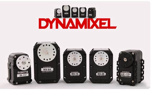
Dynamixel Servo Motors
DYNAMIXEL servo motors, made by Robotis and built around specialized robotics approaches, have a networked architecture: alongside receiving commands from the main controller, they can report back data such as position, speed, motor load, internal module temperature, input voltage, and more. Dynamixel servos can be controlled either from a computer via the USB2Dynamixel interface, or through microcontroller-based processors. Because they support full rotation, these servos work both in position-control mode, as a conventional servo, and in speed-control mode, as a motor with encoder feedback. The newer generation of Dynamixel servos (the MX series) features a 32-bit ARM processor and a 12-bit encoder, and can control motor position across the full 360° range. Today these servos are a familiar name across various RoboCup leagues - including the home robots league, rescue robots, minesweeper robots, and especially the humanoid soccer league (across its various size classes) - and they also see extensive use in a wide range of scientific and research projects.
An Integrated, Complete Servo System
DC Motor + Gearbox + Sensor + Controller + Driver + Network = DYNAMIXEL
Gearboxes
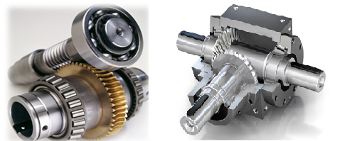
All the gearboxes used in mobile-base robots serve to reduce speed and increase torque, for two reasons: first, the DC motors used in these robots typically run at very high RPM; second, given the uneven terrain of the competition field, these robots need torque more than raw speed. These gearboxes use several types of gears, namely: spur gears, helical gears, bevel gears, worm gears, and rack gears.
Spur Gears
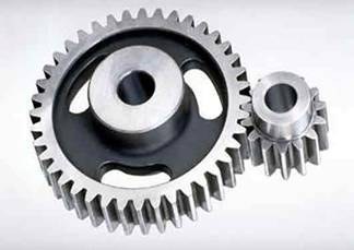
These gears are the simplest kind you'll ever see. Their teeth run straight, and the two gear shafts sit parallel to each other. Sometimes a large number of them are stacked together to cut speed and boost power. Countless devices use these gears - wind-up clocks, automatic watches, washing machines, electric fans, and more. They aren't used in cars, though, because they're noisy: every time one gear's tooth meets the tooth of the facing gear, the impact produces a small clack. Imagine the racket when a large number of these gears work together - and over the long run, these impacts eventually break the teeth. To cut down noise and extend gear life, most cars use helical gears instead.
Helical Gears
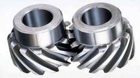
The teeth of these gears run at an angle. As one turns, the tips of the teeth make contact first, and the two teeth then gradually mesh fully together. This gradual engagement is exactly what reduces noise and lets these gears run more smoothly. Cars contain a large number of helical gears. Because the teeth sit at an angle, meshing places significant axial force on them - which is why devices using helical gears include bearings designed to absorb that force. If the tooth angle is set carefully, two helical gears can be mounted on shafts perpendicular to each other, changing the direction of rotation by 90 degrees.
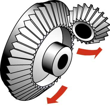
Bevel Gears
These gears are the best tool for changing direction. They're typically used for a 90-degree direction change, though they can be designed to work at other angles too. Their teeth may be straight or spiral. Straight-toothed bevel gears share the same problem as spur gears; spiral-toothed ones solve that problem, but in both cases the gear shafts must lie in the same plane. Sometimes, though, we need the gear shafts to not lie in the same plane - in such cases, we use gears like the one shown in the figure opposite.
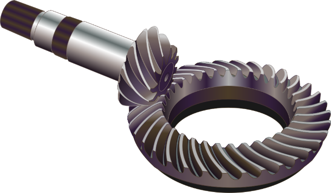
Many cars use these gears in their differential. This design lets the outer gear's shaft sit lower than the ring gear's shaft. The figure opposite shows the outer input shaft in contact with the ring gear. Since the car's drive shaft connects to the outer gear, lowering the outer gear also lets the drive shaft sit lower - meaning the shaft can be dropped, freeing up more cabin space for passengers.
Worm Gears
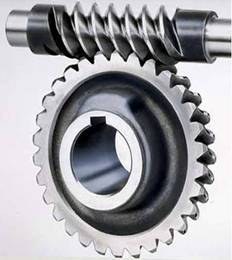
These gears are used when you need a large change in speed or power. The ratio between the two gear radii is typically 20:1, and sometimes reaches as high as 300:1 or more. These gears also have an interesting property found in no other gear type: the top gear (the worm) can easily drive the other gear (the worm wheel), but the worm wheel cannot turn the worm. The angle of the worm's threads is so shallow that when the worm wheel tries to turn it, friction becomes high enough to stop the worm from moving. This property lets us use these gears wherever a self-locking mechanism is needed. Imagine using this gear in a lift: if the lift's motor fails, the gears lock in place and keep the load from dropping. These gears are commonly used in the differentials of trucks and other heavy vehicles.
Rack Gears
These gears convert rotary motion into linear motion. A good example is a car's steering system: the steering wheel turns a gear that meshes with a rack gear. As you turn the wheel, depending on the direction of rotation, the rack moves left or right, moving the wheels accordingly. Some scales use a similar system to move their needle.
Track/Tread Width
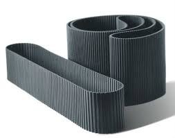
Track width depends on countless factors. It's best for a robot operating in rough or unstable terrain, such as muddy ground, to have wider tracks. Wider tracks are also recommended for heavier robots, since they hold up better under tension and won't tear under the intense forces the robot places on them. The narrower the track, the more easily the robot turns and the less energy it uses - so track width shouldn't exceed what's actually needed. The smaller the pitch (in other words, the closer the tread lugs sit together), the slower the robot's lateral movement and turning, but the more forcefully it moves - so for a heavier robot, it's better to keep the lugs close together. The author's suggestion for easing this robot's movement is to mount a row of small wheels on the track's tread, giving it behavior similar to an omnidirectional roller wheel. This robot moves easily over surfaces like ceramic tile, carpet, and grass, but struggles on high-friction surfaces such as concrete or asphalt. It's best kept lightweight, since even a small weight increase costs it a lot of capability. This robot has limited applications, and most observed examples have been mine-clearing robots.
Suspension System
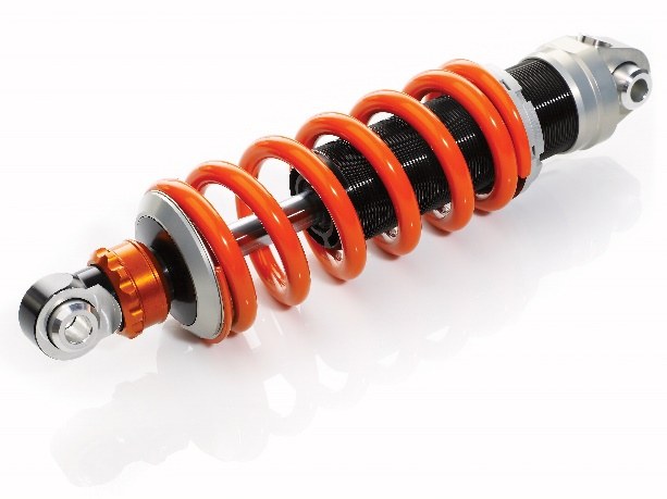
A suspension system on this robot allows for a more stable connection with the ground when meeting obstacles, letting the robot move faster, more smoothly, and more reliably over rough terrain. It's worth remembering that suspension is a relative feature, not strictly a necessity - many machines, such as most bulldozers, get by without one.
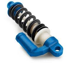
There are two main ways to implement such a system in this family of robots, described below:
The robot can be split down the middle into two separate sections joined by a hinge. This system is relatively easy to implement, but the hinge joint experiences very high mechanical stress, and the robot usually ends up damaged in this area - so the hinge joint should be built with adequate strength. The hinge doesn't have to sit exactly at the robot's midpoint; it can be offset to one side, which frees up space on the other side for mounting electronics. The idler wheels in the middle of the robot, which serve purposes other than transmitting drive power, can be linked together in pairs and move up and down in a seesaw-like arrangement.
An example is the Chieftain tank. Its rear wheel transmits drive power to the chain, while the other wheels are idlers. Except for the front and rear wheels, the tank's other wheels are arranged in pairs, each pair connected via a hydraulic system: as one wheel rises, its paired partner is pushed down by hydraulic pressure. This system works like a seesaw in the robot, and in large robots it can be implemented exactly as it is in a tank. When the tank starts moving, the rear wheel pulls its nearest neighbor upward, but because of the tank's great weight, that wheel stays on the ground instead of lifting; in a lighter robot, however, the wheel may actually leave the ground. (Note: the author has taken some liberties with the details here to make the underlying concept easier to grasp.)
Tracked robots are hazardous in many situations. If a hand gets caught between the track and the wheel, it can cause severe bruising, and in bad cases may even break or sever fingers. These accidents usually happen when the electronics and mechanical teams are working on or testing the robot at the same time. For example, in one incident we were part of, this happened just minutes before a competition began, while everyone was working on the robot at once. So mechanical team members are asked to be extra careful while their electronics teammates are working nearby, and to step back from the work if at all possible. Accidents tend to strike at the worst possible moment and can deal a serious emotional blow to the team, undermining its goals.
Methods for Designing and Manufacturing Belts
There are many ways to design and build a track/belt, but a few methods see the most use. This section covers those.
Roller Chains
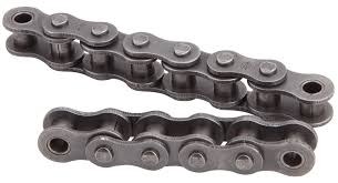
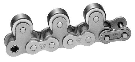
This is a very reliable and practical method, one that reduces the chance of the track coming off - one of the weak points of tracked robots - to essentially zero. That said, it doesn't offer the optimal characteristics you'd want from a track. This method uses roller chains, the kind found on bicycles and motorcycles, which come in a wide variety of models and sizes. These chains are driven by a special toothed wheel called a sprocket. The market carries an enormous range of chain-and-sprocket products, though it mainly stocks the high-demand items - which may number in the hundreds - so if the sizes you want to use in your design aren't in high demand, you'll likely have to make them yourself. It's therefore best to survey what's available before designing, and let your design follow from that. Sprockets come with or without a hub, and the hubbed type is usually more practical. Some sprockets are manufactured to a lower standard, and the chain doesn't seat properly on them - a problem especially common on smaller sprockets. So when buying, place the chain on the sprocket and confirm it seats correctly. Very small chains can slip on the sprocket under heavy load and effectively skip teeth, which wears down the sprocket, stresses the chassis, produces unwanted noise, and can damage the motors or burn out the driver circuits. To avoid this, you can use a larger chain and tension it properly during setup. Also, the more teeth a sprocket has, the lower the chance of the chain skipping.
Some chains have side plates that let you attach additional parts to them. For example, you can run two rows of chain on each side of the robot and attach plates to them to build a highly effective track.
Chains generally have some play at the pin joints connecting their links, and given the large number of links, this play adds up to a fairly significant amount - you can't safely ignore it in your calculations. The robot therefore needs a chain-tensioning capability, and you should avoid using fixed, unadjustable distances between sprockets.
Conveyor Chain
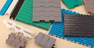
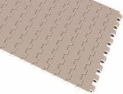
To keep the chain from slipping off the side of the sprocket, two flanges should be fitted on either side of it. For wheels meant to be idlers, a simple cylinder can serve that purpose too. Where the chain has excessive play, it generates a lot of noise, and the robot absorbs significant vibration. To eliminate this, you can fit rubber or polymer segments - such as wear-resistant belt material or polyurethane - onto each chain link. Including a chain-tensioning system in the design is recommended. Some of these chains can also flex sideways, not just at the hinge - a capability that's a liability for most designs and is best avoided.
Thermal Belts
It's recommended to use versions without a reinforcing cable, since this makes splicing the belt and mounting it on the robot much easier.
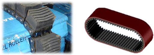
To splice this type of belt, simply heat both ends with a clean flame - such as a gas stove or lighter - until they melt, join them together, then patiently wait for the joint to cool. Because these belts conduct heat poorly, thicker belts take longer to cool at the joint, so be extra patient with them. To speed up cooling, you can use an ice-water mixture. Any excess material at the joint can be trimmed off with a utility blade and smoothed with sandpaper. This type of belt has low friction against the ground, so for professional applications it's recommended to use other belt-manufacturing methods instead. Suitable pulleys for this belt are simple cylinders fitted with circular grooves.
O-Rings
For small, non-professional robots, O-rings can be used in place of a track. O-rings come in standard sizes, so the robot must be designed around whichever O-rings are available on the market. A robot built this way ends up with a structure similar to one using thermal belts.
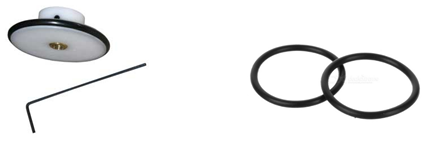
Automotive Belts and Pulleys
In car engines, wheels and belts are used to transfer power. These belts have high tensile strength and typically carry power from the engine to the alternator and one or more pumps. These belts and their matching pulleys come in standard sizes on the market. Some of these belts are fairly thin and need to be built up with another flexible layer to reach the desired thickness.
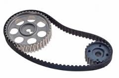
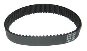
The drawback of this method is that using these belts limits the design, since belt and pulley sizes are fixed - the designer ends up building the robot to suit the belt, rather than choosing the belt to suit the robot. Its advantage is lower cost, and in areas where builders don't have access to specialized track material, it makes it possible to build semi-professional robots.
Timing Belt (Synchronous Toothed Belt)
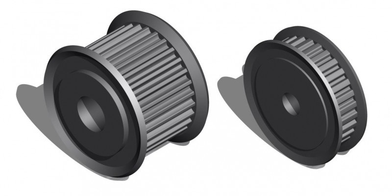
Double-Sided Belt
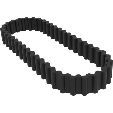
This is a variant of timing belt with teeth on both sides. Its use case is quite narrow, though, so finding an acceptable range of it is also difficult.
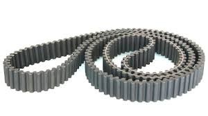
Combining Timing Belts with Other Belts
In this method, an extra layer is added to the outer surface of the timing belt - this layer can be rubber foam, a rubber belt, or any other covering. There's a specific product on the market, branded as wear-resistant belt, that suits this purpose particularly well. It comes in 4 mm and 6 mm thicknesses, and its outer surface offers very high friction with surfaces it contacts - enough that, like an adhesive, it clings to smooth surfaces. If you press a piece of it against a pane of glass for a moment, it stays stuck to the glass after you release the pressure, instead of falling off. One side of this belt is smooth, while the other has fine ridges that help it bond, with a special adhesive, to the outer surface of the timing belt. It's also quite flexible and doesn't create the problems typical of stiff coverings. For most applications, wear-resistant belt has no real rival among the alternatives. Some robot builders mount the ridged inner surface facing the ground and glue the smooth surface to the timing belt - this results in poor adhesion between the two belts, and the rough surface also picks up dirt quickly in messy workshop environments. Sellers typically handle the entire process of assembling the two belts together. Paying attention to three points keeps the manufacturing process trouble-free; ignoring them leads to heavy losses of both time and money. First, the wear-resistant belt itself might be degraded - something you have no way to spot yourself. Degraded belt material doesn't bond well to the timing belt and may separate under pressure; it also tends to develop countless tiny cracks over time. To avoid this, work with established sellers rather than unknown vendors just to save a small amount of money. If a seller explains the price difference between degraded and sound belt stock and walks you through sample comparisons, you can trust their work more. Second, the seller may lack experience assembling timing belt with wear-resistant belt and unknowingly use the wrong adhesive for the job. To guard against this, order a small test sample first, then try to pry the two belts apart with a tool like a screwdriver - in a good bond, the wear-resistant layer will tear under this test before it separates from the timing belt. During manufacturing, a strip of wear-resistant belt is glued onto the timing belt, and the two ends of the strip are also glued to each other. To ensure the joint holds firmly and doesn't come apart, the joint's contact length needs to be increased - done by cutting the two ends at a shallower angle instead of a 90-degree cut. There are other methods for achieving this too, and you can ask belt suppliers for the details.
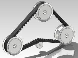
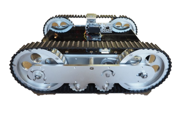
If your robot is built to move on carpet, use grip belt as the covering instead of wear-resistant belt for better results. Small strips of wear-resistant belt should be attached across it so the surface has small steps, improving how well it grips the terrain. It's best to keep these steps close together, otherwise the robot will experience a lot of vibration and bouncing. The strips can be mounted at an angle across the belt - but if the robot needs to climb stairs, avoid doing this. If the robot is heavy, use a wider belt, since excessive pressure could tear it.
There are two different variants of this belt, as follows:
The first type is mainly used in snowmobiles. In this design, two rubber belts are connected by metal rods, with a fixed gap between them. The teeth of the vehicle's drive sprocket engage the gap between the belts, meshing with the metal rods. The vehicle's weight is transferred onto the belt through rubber wheels. The metal pieces on the belt keep it engaged with the wheels and prevent it from slipping off. Robots using this method need a belt-tensioning mechanism.
This method is widely used both in snowmobiles and in robots. It lets us build robots that essentially run on wheels but can be converted into tracked robots whenever needed. Typically, in this method, there's one belt strand on each side, with metal pieces attached to it that keep the belt stable. The robot's drive power is transmitted to the belt through the wheels - ideally, drive power should be transferred to the track through more than one wheel. Robots using this method don't strictly need a belt-tensioning mechanism, though one may still come in handy depending on the situation.
There are countless ways to design and build this belt and its metal fittings - discovering them is left to your own resourceful thinking. To join the two ends of the belt, you can splice them together; as mentioned in the section on combining timing belts with other belts, you need to angle the splice joint rather than cutting it straight across. Another approach is to make the belt slightly longer, overlap its two ends, and then bolt the overlapping edges together using metal plates and hardware. Robots that run on these belts experience a fair amount of vibration; to reduce this, use more metal pieces spaced closer together.
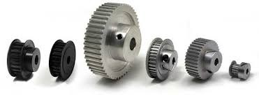
Using Simple Rubber Belts
You can splice the two ends of a simple rubber belt together and use it directly on the robot. It's best if the robot's drive wheel is large, so a wide arc of the wheel stays in contact with the belt. All drive and idler wheels need flanges so the belt doesn't slip off. To improve contact between the wheel and belt, you can coat the wheel with something like silicone paste, wear-resistant belt material, or a similar covering. Build a belt-tensioning system into the robot. Don't over-tighten the belt, since that invites problems, one of which is the belt tearing. Fiber-reinforced rubber belts are recommended.
Manufacturing Specialized Belts
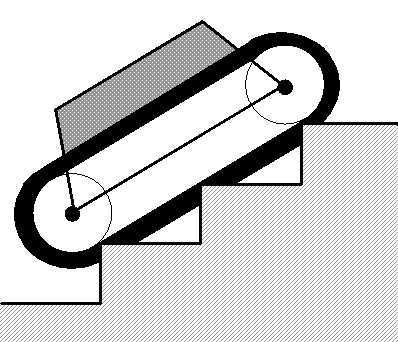
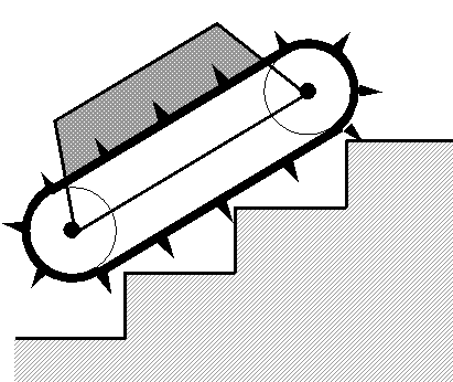
This method is used for robots designed for mass production. The track on this kind of robot is designed precisely to match the robot's performance, and manufactured in special molds that vary depending on the track type. A few points need the designer's attention when designing this kind of track:
Belt thickness depends on two factors: the required tensile strength and its flexibility. The thicker the belt, the less flexible it is - and that costs the robot some of its energy during movement.
The external lugs on the belt are designed to match the environment the robot operates in. If the robot needs to climb stairs, horizontal lugs work better; otherwise, angled lugs are more suitable, since they cut down on vibration during movement and let the track engage the terrain more effectively. There are two types of ridges on the belt's inner surface: one lets the belt engage the wheel so drive power transfers to it, and the other keeps the belt from slipping out of place - this second ridge usually runs along the belt's center.
This robot's wheels are designed and built to match the lugs on the belt. To join the two ends of metered O-ring cord, it's best to use Loctite or a similar adhesive along with special rubber-bonding compounds. O-rings are quite inexpensive and can be bought from sellers who also supply bearings and oil seals. To take advantage of an O-ring's sealing property, a groove needs to be cut at the leak point for the O-ring to sit in. Reference tables exist for designing the groove's dimensions, and you should pull these from the internet before starting your design.
Wear-Resistant Belt
Wear-resistant belt is a special type of belting with extremely high friction against surfaces - far higher than rubber or polyurethane. If you press a piece of it lightly against a vertical pane of glass, it clings to the glass like an adhesive, and, as you'd expect, it shows this same tenacious grip when it meets terrain. This belt has two faces: one covered in fine ridges, and the other smooth. The ridged surface actually has lower friction than the smooth one and is used for attaching the belt wherever needed - some people mistakenly assume the ridged surface has more friction and end up designing around that wrong assumption. You can bond this belt onto the surface of the robot's wheels or tracks, and you can also apply a bit of it to the robot's gripper fingers to improve their grip. This belting is highly elastic and very flexible, so it can't be used alone as a full track. If you stick a small strip of it under a box, you can be sure the box won't slide off a table. If this belt is used on the outer layer of a robot's wheels or track, it increases the robot's energy consumption and places a heavy load on the motors during movement - so the motors need to be powerful enough not to be overwhelmed by the belt's friction. This friction is very useful for the wheels of robots like combat robots that push against each other, and robots like rescue robots, which tackle very steep slopes, simply can't succeed without this material. This belt is generally available in two thicknesses - 4 mm and 6 mm. The 4 mm version is cream-colored, and the 6 mm version is red. These belts don't come in standard widths; the seller cuts them to whatever width you need. Their length isn't standardized either, and they're cut by the meter as needed. Cutting this material is somewhat tricky, so it's best left to the seller. Over time, this belt degrades, and both degraded and sound stock get sold at different prices in the market. The two look identical, but degraded belts crack within a short time and become unusable. Buy only from a trusted seller, since you can't tell degraded material from sound material yourself. The bonding surface should never be polyamide, Teflon, ABS, or similar materials, since adhesive doesn't bond well to them and the joint won't hold properly. Once you've bonded the belt onto a wheel or track, you also need to glue its two ends together - and this joint must be strong enough that it never comes apart. To achieve that, the two ends should be cut in a way that maximizes the bonding surface area. Three of the various methods for doing this are illustrated in the table below:
Roller Chains and Sprockets
Chain, together with its matching sprocket, is used to convert and transmit power, and in robotics it's used for power conversion, power transmission, and building tracks. These chains resemble bicycle chains and come in a wide variety of sizes and designs. A chain draws power from one toothed wheel - a sprocket - and transfers it to another sprocket. Roller-chain sellers typically stock a wide range of sprockets. Despite this broad selection, some items aren't available in these shops, and others are in very short supply, so when designing, check the market first so the robot's design doesn't drift too far from what's actually available. Some sprockets aren't made to an acceptable standard, and the chain doesn't seat well on them - so before buying, make sure the chain fits the sprocket perfectly. Sprockets come with or without a hub. If you buy hubless sprockets, you'll likely need to machine and weld a hub onto them yourself; not all sprockets lack a hub, though, so check the market during the design phase. Hubbed and hubless items are priced the same, and only in rare cases does the price differ.
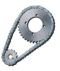
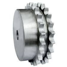
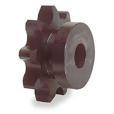
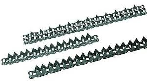
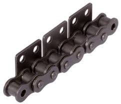
Some chains are double-row, and their breaking strength is higher than single-row chains of similar dimensions. Some chains have side plates that let you mount components onto them. Because of play between the links, a chain's length isn't fixed - pull it taut with even a small force, like your hand, and it reaches its maximum length. Suppose you have two seemingly identical chains from two different manufacturers: their maximum length over 100 links will still differ. What this means for us is that a chain running back and forth between two sprockets might end up too short and refuse to seat properly, or too loose and cause problems. Designing a system where the chain sits neither too loose nor too tight, but seated optimally, is difficult. The fix is to run the chain slightly loose and use chain-tensioning mechanisms to adjust its tightness. There are various ways to do this, including:
- Making the distance between the two main sprockets adjustable.
- Having a small gear press down on the chain from above.
- Having a plastic or rubber roller press down on the chain from above.
In some cases, chains skip teeth under load - meaning the chain slips between the teeth, produces an abnormal noise, and can damage the sprocket or the robot's chassis. There are four solutions to this problem:
- Using a double-row chain, or a chain with two or more rows.
- Using a larger chain-and-sprocket size number.
- Using sprockets with more teeth.
- Tightening the chain.
Another advantage of chain is its ability to convert power ratios. To do this, the sprockets engaged by a single chain carry different tooth counts. The chain draws power from one sprocket and transfers it to another; the ratio between the driven sprocket's tooth count and the driving sprocket's tooth count is the transmission ratio for that stage. If power passes through several stages - in other words, if there are multiple transmission stages - the overall transmission ratio is the product of all the individual stage ratios.
Timing Belt
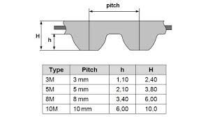
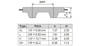
Some friends and machinists, unfamiliar with how to actually make this pulley, recommend methods like wire EDM or extrusion. Our recommendation, though, is machining it on a milling machine. That said, no ready-made cutting tool exists in the market for cutting these gear teeth, so you'll need to make the tool yourself - one way is by hand-grinding a cutting blade and mounting it to a shaper. Another approach is to have a toolmaking and tool-sharpening workshop machine a precise rotary cutter for you. Because the process for making a timing pulley differs from other gears, manufacturing costs run somewhat higher. To find machine shops skilled at making this gear, ask belt suppliers for recommendations. To make a timing pulley, you can use materials such as dry-machined aluminum, polyamide, or ABS. Pulleys tend to be quite heavy, so to save weight, drill them out or bore out their interior.
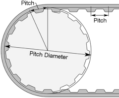
There are formulas for calculating tooth count and outer diameter, but the table below covers a good range of requirements well, and machinists are generally more familiar with this table than with the formulas. One unpleasant issue that comes up with this system is the belt coming off the pulley. This can happen for several reasons, including:
- Over-tensioning the belt from too-tight adjustment
- The belt edge catching on the pulley flanges
- Misalignment between the two pulleys' rotation axes
- Poor manufacturing quality of the pulley
- A defect in the belt
Ways to prevent these problems include:
- Adding one or more guide pulleys to the system
- Using a wider belt
- Loosening the belt tension slightly
- Chamfering the edges of the pulley flanges
A timing-belt system is also used to convert rotation ratios. It's recommended to base your ratio calculations on the pulleys' mean diameter as the primary reference; where possible, though, it's better to use tooth counts instead. The belt behaves exactly the same way as roller-chain transmission ratios do.
The belt's tension needs to be adjusted properly: too loose, and it slips over the pulley teeth - in other words, it skips teeth; too tight, and it lowers the belt's tear threshold, stresses the chassis and other components, and increases energy consumption. There are several ways to tension a belt, some of which are covered below:
- Making the distance between the pulleys adjustable
- Installing an extra pulley to adjust belt tension
- Installing a cylindrical wheel above the belt that presses down on it
In a timing-belt system, more than two pulleys often engage a single belt at once. In many of these cases, one pulley is a pure idler - it neither drives the system nor draws power from it. To save cost and weight, these pulleys shouldn't be toothed; make them fully round instead, with a diameter matching the root diameter of the toothed pulleys - in other words, use a plain cylinder in place of a timing pulley. For transmitting power to pulleys in robots like omnidirectional-wheel robots, avoid using timing belt as much as possible, since tensioning multiple belts is a manual process, and they never end up tensioned exactly alike.
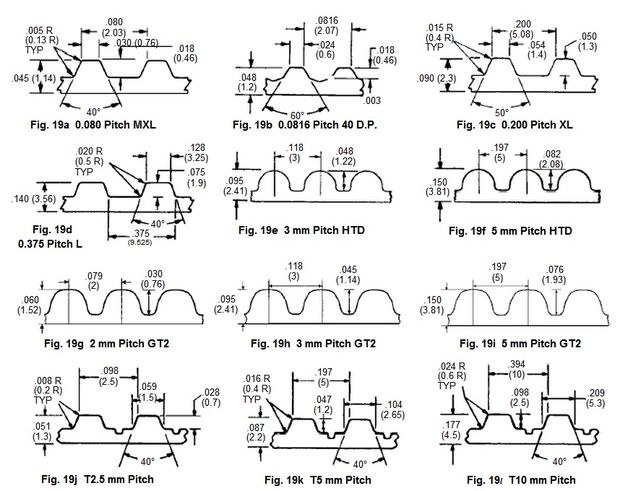
Ball Bearings
Ball bearings, or rolling-element bearings, are such a familiar concept that defining them isn't really necessary. Bearings come in an enormous range of structures, with classification schemes spanning at least thirty categories. Given the scope of this book, covering the full classification and coding system for bearings isn't practical. In industry, single-row ball bearings see more use than other types and are easier to find in a wide range of sizes.
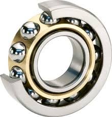
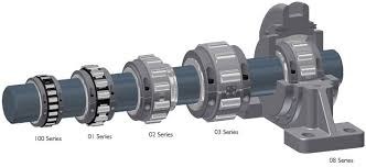
Rolling-Element Bearings
Rolling-element bearings cover a broad concept, but the text above focuses mainly on documenting what's available in the market rather than diving into the underlying theory.
- The shaft sits perpendicular to the bearing's mounting face, and two bolts are used to attach it.
- The shaft sits perpendicular to the bearing's mounting face, and four bolts are used to attach it.
- The shaft sits parallel to the bearing's mounting face, and two bolts are used to attach it.
- Other bearing-housing types see less use and are rarer in the market.
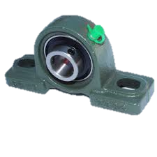
Plain (Sliding) Bearings
Plain bearings work like a door hinge: a round rod rotates inside a hole, with the rod's outer surface sliding directly against the hole's inner surface.
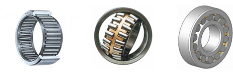
Bolts and Nuts
In industrial robots, bolts and nuts are mainly used to join parts together. Bolts come in many shapes, each suited to a particular situation. If we classify the most common bolts by the tool used to drive them, we should mention slotted, Phillips, hex-socket (Allen), and multi-sided (hex-head) bolts. Slotted and Phillips bolts are driven with a screwdriver and cost less than other types. Hex-socket bolts are tightened with an Allen wrench, and the authors prefer them over other types in most situations, though they cost more. Multi-sided bolts are tightened with a wrench, and the most common of these is the hex bolt, widely available at reasonable prices.
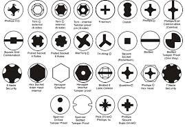
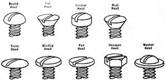
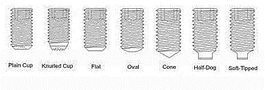
In terms of sizing and how they're sold, the bolt market splits into metric and imperial (inch-based) types. Imperial bolts have finer threads, are scarce and expensive, and overall aren't something you can reliably count on.
Bolts come in a wide variety of head shapes - that is, the raised feature at one end. That said, ordinary pan-head, set-screw (headless), and countersunk bolts are the most common. Ordinary bolts have a raised head, either cylindrical or multi-sided. Many designers forget to include bolt heads in their design models and only discover during manufacturing that the head collides with other robot components, running into trouble as a result. Set screws (grub screws) have no head at all - the entire body is threaded. These aren't used for joining parts together; instead, they're used for things like locking a shaft in place inside a hole. Some designers make mistakes when using these screws to fix a shaft inside a hole, choosing screws with too small a diameter and running into problems: a narrow-diameter screw can't be tightened very much, so its tip applies little force to the shaft, and the shaft doesn't get properly locked in place. These screws thread directly into a tapped hole and never see a matching nut on their own body. Countersunk screws have a conical head and are used where the head must sit flush with, or below, the work surface. Before installing these screws, the top of the hole is first countersunk - using a large drill bit or a countersink bit - so the head can seat inside it. Bolts are usually made of steel and have relatively low hardness; they're generally vulnerable to rust, though some are blackened or plated to resist moisture better. If a bolt needs to withstand harsh chemical or mechanical conditions, titanium bolts are the better choice - though they're expensive and hard to find. Stainless steel bolts make a good, accessible second choice.
Some bolts are known as "threaded rod" - essentially a one-meter rod threaded along its length, with no head or similar feature. When you need an unusually long bolt, or a bolt in a length that doesn't exist as a standard size, threaded rod comes in handy: you saw off whatever length you need and lock it in place with nuts on both ends. Another use for these rods is emergency situations where there's no time to work out the exact number and size of bolts needed - in these cases, you just buy a few lengths of threaded rod and use them as needed. Threaded rod isn't made in diameters smaller than 4 millimeters. Short bolts are threaded along their entire body, while long bolts are only threaded along a limited portion near the tip. Many people thread bolts directly into tapped holes in a part - this simplifies the design process, but stress on the bolt can damage the threads, forcing you to repair or replace the part. So it's recommended to use a bolt-and-nut combination wherever possible and avoid over-relying on tapped holes in parts. Also, blow out the threads with compressed air before installing a bolt. A nut is a part with a threaded hole through it, tightened in place with a general-purpose or specialized wrench. Most nuts are hexagonal and tighten with an ordinary wrench. Many nuts sold in the market are of poor quality, so check their quality by test-fitting a bolt at the time of purchase whenever possible. Try to buy plated nuts, since they hold up better against moisture and chemical exposure. Some bolts are known as "wood screws" (self-tapping screws); these have no matching nut and are suited to driving into wood, plastic, wall anchors, particleboard, and MDF. In robotics work, you can use these screws to attach parts to plastic sheets such as polyamide. In some cases, no pre-drilling or tapping is needed at all, and the screw can be driven straight into the target material. Before buying small screws, we recommend confirming that a matching wrench or screwdriver is actually available in the market. There are several ways to keep a nut from loosening on its own, ranked here by effectiveness:
- Apply a specialized thread-locking adhesive inside the nut - these adhesives are introduced in the relevant section.
- Instead of one nut, tighten two nuts together (a jam-nut setup), and torque both down firmly.
- Place a spring (lock) washer and a flat washer under the nut.
- Some nuts have a built-in rubber ring and won't loosen on their own (nylon-insert lock nuts).
Couplings
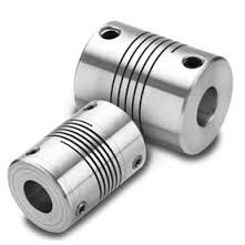
This part can serve many purposes, but it's typically used to transfer power from one shaft to another. For example, you might want to measure a shaft's rotation - to do this, you connect the shaft to a rotary encoder sensor using a coupling.
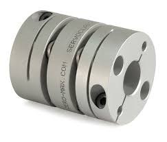
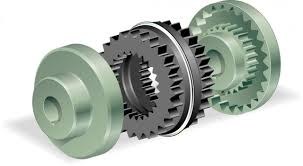
Retaining Rings (Circlips)
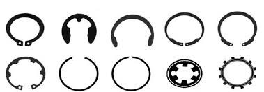
Generally speaking, using a circlip to fix shafts, bearings, and similar parts in place leaves a small amount of play, which isn't ideal for certain applications - so for very precision-critical work, it's best to avoid this method. The authors' own design approach avoids circlips altogether, but since they're so widely used by robot builders, they're covered here anyway.
For a circlip to sit properly on a shaft, the circlip's inner diameter needs to be slightly smaller than the shaft, and the shaft needs a groove matching the circlip's diameter. The circlip is spread open using a tool called circlip pliers and springs into place in the groove. For a bore (internal) circlip, its outer diameter is slightly larger than the hole, and the hole has a matching groove for the circlip's diameter. The circlip is compressed using a tool called internal circlip pliers and drops into place. When a bore circlip is compressed, its opening measurement is d4; when a shaft circlip is expanded, its opening measurement is d4. One of the biggest mistakes some builders make when using circlips is ignoring this d4 measurement, designing the assembly in a way that leaves no room to open or close the circlip pliers, making installation impossible. Another mistake is using shaft and bore circlips right next to each other, which likewise makes assembly difficult, and sometimes impossible.
Overview of Part-Manufacturing Techniques
Manufacturing is the process of turning raw materials into a finished product, encompassing the design and fabrication of objects using a range of techniques. This definition covers an enormous scope - everything from shaping large metal parts using explosive forming to stitching with a sewing machine, along with countless other processes and tools.
This chapter aims to introduce the manufacturing processes most widely used in robotics. That said, reading this chapter - or even specialized manufacturing textbooks - will only give you a general outline; the manufacturing mindset doesn't truly take root until you've worked hands-on with these methods and had parts you've designed actually made through various processes. If you can gain experience at machine-building companies or large machining workshops, you'll come to understand the real substance of manufacturing, along with its risks and limitations.
Simplification
Parts should have a simple structure. Designing complex parts increases the odds of mistakes. It's also better for the overall design to stay simple, since complexity increases the chance that some detail in the design or execution will run into trouble.
Reducing Part Variety
Turning (Lathe Work)
The lathe is one of the oldest machine tools. To understand how it works, picture a pencil held and spun in your hand as the workpiece, with a pencil sharpener shaving its surface. In turning, the workpiece is clamped in a special fixture called a chuck, and if it's long, the other end is supported by a tool called a tailstock (live center). Rotating the chuck spins the workpiece. The cutting tool is mounted on a tool holder (the carriage), which moves at a steady rate along the workpiece's axis, in front of it, removing material as it goes.
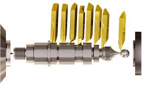
Round objects are generally made using turning. The turning process serves many purposes, and you can produce a wide range of shapes with it. Some of the operations performed on a lathe are as follows:
Turning: straight, tapered, contoured, and grooved shapes, such as shafts, axles, pins, handles, and similar parts.
Facing: flattening the end face of a workpiece.
Form turning: complex profiles, such as curves, can be ground onto the cutting tool, and that same profile is then imparted onto the workpiece during turning.
Boring: enlarging a hole that was already created by another process, or cutting an internal groove.
Drilling: creating a hole, which then comes out smoother and more precise through boring.
Parting off: separating or cutting off a section from the end of the workpiece.
Thread cutting: creating internal or external threads on the workpiece.
Knurling: creating a regular, textured pattern on the surface of cylindrical parts, such as handles.
Tapping: creating threads inside a hole.
Reaming: improving the precision and dimensions of a hole using a specialized tool.
Filing: while the workpiece rotates, a file is held by hand against its surface.
Grinding: a special rotating grinding wheel brings the workpiece's surface to precise dimensions.
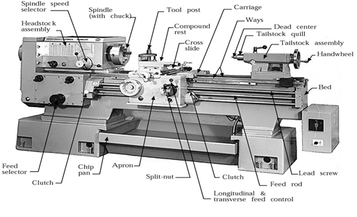
Milling
This process encompasses a range of multi-purpose machining operations capable of producing a wide variety of shapes. A milling cutter has several cutting edges, each removing a chip with every rotation. Generally, both flat and contoured surfaces can be produced this way. This method can also be used like a drill to create holes. Ball-nose (hemispherical-edge) tools are used to produce curved surfaces in mold-making. The first milling machine was built in 1876. Because of their ability to perform such a wide range of operations, milling machines rank among the most important multi-purpose machine tools. On most common milling machines, the cutting tool rotates in a fixed location, while the workpiece moves relative to the tool via a table that travels horizontally and vertically. Auxiliary fixtures can be mounted on the table - for example, a chuck, a rotary table, or a tilting table, letting you change the workpiece's orientation or angle relative to the machine. Making parts such as gears, keyways, multi-sided shapes, and complex curves is among the most common work done on a milling machine.
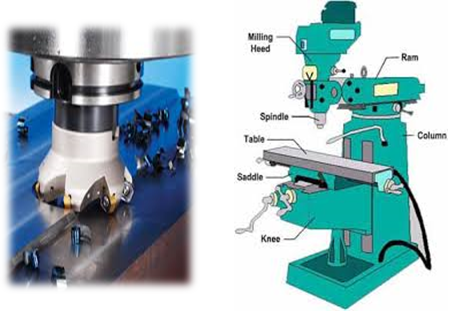
Hobbing Machine
This is a specialized type of milling machine dedicated to making gears. It improves gear quality while cutting manufacturing time and cost. It's recommended to avoid building your own gearbox and instead take advantage of the wide range of ready-made gearboxes available. If you have no choice but to build one, allow proper backlash between the gears, and design a rigid, reliable housing for the gearbox. It's also recommended to draw on the experience of skilled gear-cutters.
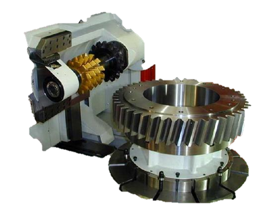
CNC
In the evolution of manufacturing machinery, NC (numerically controlled) machines came about. These machines carry sensors such as linear and rotary encoders. Using these sensors, the exact position of the tool or workpiece, along with its coordinates, is displayed on the machine's control panel. In essence, it's still fundamentally a manual machine, except the numbers are read off a monitor instead of a vernier scale. On these machines, the error that would otherwise come from play in the machine's components is reduced to a minimum. Their precision runs around one-thousandth of a millimeter. Working with these machines is reliable and genuinely enjoyable. Today they're used extensively, though they carry a steep price tag. Machines such as the rotary tool ("super drill") are typically built around this mechanism.
The next wave of progress came with the arrival of CNC machines. In terms of sensor architecture, these are similar to NC machines. A handful of small motors, connected to classic mechanical structures, adjust the relative position of the tool and workpiece, with the whole system directed by a computer. The machine operates based on a predetermined program stored in the computer's memory, guided and controlled using sensor feedback together with the control motors; machines such as wire EDM units fundamentally run on this same system.
The cost of CNC machining is calculated based on machine time. The most common of these machines are CNC lathes and CNC mills. To place an order for CNC work, bring along an AutoCAD file with 2D drawings of the part; when drawing, avoid the SPLINE command and build curves out of multiple ARC segments instead.
EDM (Spark Erosion) Machine
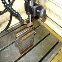
After the lathe, mill, and pillar drill, the EDM machine, with its fascinating mechanism, is the next most common machine found in machining workshops. It works on the principle of electrical discharge: bringing the two ends of a current-carrying wire close together produces an electric arc, which erodes away a tiny bit of metal and leaves behind a small cavity. Electrical discharge machining was developed in 1940.
In this method, the electrode plays the role of the cutting tool. An electric potential difference is set up between the electrode and the workpiece, producing tiny electric arcs between them. These sparks erode away material from the workpiece's surface. The workpiece and tool sit about 0.01 millimeters apart. A dielectric fluid - which can be kerosene - flows between the workpiece and the electrode, acting as an insulator, flushing away debris, and cooling the workpiece. The electrode can be shaped however you like - for instance, you could make a square-shaped tool to cut deep holes with a square cross-section. Electrodes are usually made of copper, though they can also be brass, graphite, or tungsten. Some metals machine easily under spark erosion, while others, such as copper and titanium, are more troublesome; for these metals, use electrodes other than copper and its alloys. The material-removal rate for these metals is quite low. On an EDM machine, the tool is lowered via a device called a servo mechanism. The higher an electrode's melting point, the lower its wear rate - which is why graphite has the lowest wear rate of all. By adjusting the potential difference and current, you can raise or lower the material-removal rate: at a lower removal rate, the work comes out more precise. This process places no mechanical stress on the workpiece, so it doesn't experience fatigue. That said, at a high removal rate, repeated melting and re-solidification of the metal disrupts the surface's uniformity - a flaw you can correct afterward through finishing.
Wire EDM
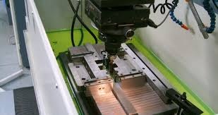
In most jobs, the raw material is a thick metal sheet. Before starting the wire-EDM process, check that the top and bottom surfaces of the sheet are parallel; if they aren't, flatten them using methods such as magnetic grinding. Clean the surfaces thoroughly before handing the raw material over to the wire-EDM shop. Don't use warped sheets, and when buying raw material, avoid cutting methods like plasma, oxy-fuel, or guillotine shearing, which introduce warping into the part. Ignoring these points can damage the part, or the wire-EDM shop may simply refuse the job. Before starting wire EDM, a hole is drilled into the part - using a drill or rotary tool - and the wire is threaded through it. Given the high volume of work at wire-EDM shops, your job could easily get forgotten, so follow up regularly on its progress. On the part, the wire-EDM cut starts at one point and ends at another; a small burr is left behind at the end point, which can interfere with the work. To prevent this, mark the start and end points of the cut in advance and let the operators know. Vibration in thin sheets during wire EDM, caused by the dielectric flow, can also cause problems - operators can recommend various ways to fix this. To wire-EDM cut several sheets together, first clean them, stack them on top of each other, and clamp them with a few small clamps, such as a hand vise. After that, weld the edges
together. If any weld splatter reaches the top or bottom surface, remove it by grinding.
3D Printer

3D printers are devices that let you turn images on your computer into real, physical three-dimensional models. The technology used in newer 3D printers lets users incorporate composite materials into their designs for 3D printing. A 3D printer can print your computer designs as a real object with very high precision. 3D printing technology is advancing rapidly and can print computer designs as physical three-dimensional objects. Today, 3D printing has caught on not just as a hobby among everyday users - fields such as medicine and industrial modeling have embraced it too. It seems likely that, in the future, the largest group of 3D-printer users will come from the developing world, since the scarcity of certain resources and tools opens up room for producing them with this kind of printer. RepRap introduced the first home 3D printers. Home 3D printers generally produce objects by melting plastic, while industrial 3D printers have been built that can print using metals, liquid resins, ceramic paste, and even food materials. It's been less than a decade since laser printers took over and dot-matrix printers fell out of use, and you could say that during that stretch, the stunning quality of laser printers kept every user satisfied - yet no one predicted that, in under ten years, printers would appear on the market that laser printers simply couldn't compare to. From here on, whatever you can imagine and design as a 3D model on your computer, you can hold in the physical world within minutes. 3D printers are also known as additive, or layer-based, manufacturers, since their basic method is building up the desired object layer by layer until it reaches the final requested shape. This method's biggest advantage over traditional approaches is higher precision, greater speed, and far less waste of raw material.
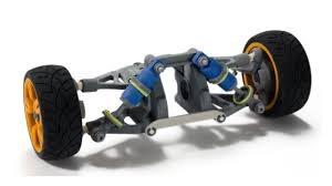
As for the applications of these printers, they're already serving many industries today, though at a very small scale within those industries. Because of how demanding their control and operation are, 3D printers are typically used to build prototypes of products rather than for use on factory production lines. Today, with technology companies becoming active in this space, we're seeing home versions of these printers being built - though they still haven't really found their footing among home consumers the way they should. Now take a moment to imagine what you could do if you owned one of these! Instead of buying certain products online, you could produce the item you want, with whatever custom tweaks you like, right in your own room, and enjoy it.
Introduction to 3D Printers
Printers, which have been part of people's everyday lives and technology for some time now, and which see very heavy use, are devices for printing information and images onto paper - sometimes in color via laser, and sometimes via the older dot-matrix method. But 3D printers are a fascinating kind of printer that, using composite materials, can build and deliver any image you want as a physical three-dimensional object. These printers, which are in especially high demand these days and carry a hefty price tag, have amazed everyone. At this year's CES 2014, several types of these printers were introduced to the public, working with a range of different materials and offering the ability to build and print at higher speed and greater volume. In their early stages, these printers are mostly used to build models and objects people want, offering high-resolution help to users; more advanced designs of this kind of printer, using a wider range of materials, can produce objects that are more realistic and match the intended sample exactly - though these devices are still in their early design stages, with only a handful of units produced so far.
3D printers have been used commercially in various industrialized countries for several years now. Today, 3D printing is used to make precise, complex parts for models, which has boosted both the speed and accuracy of part production. Building a model part via 3D printing requires preparing a 3D file of the part in question; the machine reads this file and builds the object by laying down material in stages, layer by layer. A 3D printer is, in effect, a printer that, besides producing a pattern in length and width, can also print vertically. Imagine, for instance, that the printer's "ink" is a hundredth of a millimeter thick, and you want to produce a cube-shaped part, like a sugar cube, in three dimensions. The printer starts by printing a roughly one-by-one-centimeter square at a thickness of a hundredth of a millimeter. Once this layer is done, the nozzles that dispense the material move up slightly and print another layer on top of the previous one. This repeats until you end up with a complete three-dimensional cube. The only difference with actual 3D printers is that they can use materials such as various plastics and resins to build parts, and the layer thickness is larger than a hundredth of a millimeter - typically around a tenth of a millimeter, considered the ideal thickness. Layering speed, layer thickness, and the material used are all important factors in the quality and accuracy of the finished part. Parts produced this way usually don't have a great surface finish and need some post-processing before they're presentation-ready. As for how these machines work, and their fundamental difference from CNC machines: 3D printers mainly build the final product by depositing molten material, whereas CNC machines mainly reach the final product by cutting away, or removing, material from a larger block. That said, operating either machine requires proper training - otherwise, neither is easy to use. 3D printers, though, work differently depending on their input material: some work with plastic, nylon, metal, or other flowable materials, depending on what we need from the final product. After melting the raw material, 3D printers inject it layer by layer onto a build platform; these layers bond firmly to one another, and after a short time, our finished product is ready to use.
The Value of 3D Printers
The real value of these printers can be examined from two angles: economics and innovation. From an economic standpoint, this kind of printer opens up new economic opportunities for society - with their help, the speed and variety of product manufacturing increase, and so does quality, which in turn creates thousands of job opportunities for society. Now imagine having a machine at home that can pull your dreams and ideas out of the imaginary and virtual world and into the real one, letting you actually see your thoughts take shape! In that scenario, it would undoubtedly spark a kind of revolution in innovation and manufacturing, since from that point on, the cost of turning an idea into reality drops dramatically. For example, instead of going to a store to buy shoes, you could find a 3D file sized to fit you on the internet, buy it for a lower price, then print it and start using it!
Applications of 3D Printers
Today, 3D modeling is common across a wide range of fields - parts manufacturing, architecture, industrial design, robotics, aerospace, and more. Until recently, these models were presented as two-dimensional images on a screen or on paper, so people could look at them and get some sense of what the designers had in mind. As for 3D printer applications across various industries: unfortunately, most new technologies are born out of the military-industrial complex, and 3D printing technology is no exception - it first emerged in the manufacturing of military parts. After a while, though, applications of this technology spread into other industries. These applications typically arise where a part is highly complex, or where a prototype is needed for modeling purposes.
Rotary Tool (Super Drill)
This machine essentially works like a spark-erosion EDM machine. That said, its electrode is a thin rod, usually one to three millimeters in diameter. This rod spins about its own axis and descends onto the workpiece's surface.
For producing small, deep, precise holes, this machine is the best method available and commonly used. Its material-removal rate is high, and it works quickly. Unlike long drill bits, which deflect during drilling - causing the exit point to end up off from where you actually wanted it - that doesn't happen with this method. With this machine, you can create holes exactly where you intend. These machines are generally NC-controlled.
Sawing
Sawing is a process in which the cutting tool is a blade lined with a row of small teeth, each of which shaves away a small amount of material from the workpiece. This process works on virtually any metallic or non-metallic material that's machinable by other methods too. The cutting kerf in sawing is generally narrow, so material waste from sawing stays low. In building robot parts, you may run into several types of saws, introduced below:
Hand Hacksaw
This saw is used for cutting machinable metals and polymers. It consists of a frame (bow) with a replaceable blade attached to it. These saws cut on the forward stroke, so this needs to be kept in mind when mounting the blade in the frame. Also, buy blades that are flexible enough to bend without snapping. Some of these saws are small enough to fit easily in your toolbox. There are also special "blades" that are really just rough rods - these are used for cutting glass and hardened metals that can't be machined by other means.
Power Hacksaw
This saw has a structure similar to the hand hacksaw. In this machine, the blade's back-and-forth motion is powered by the machine itself, and the cutting area is cooled with a soap-and-water solution. Some of these saws use a band-type blade and run at higher speed. This machine is used to cut round stock, multi-sided profiles, machinable metals, and polymers, and comes in various sizes and power ratings. In some cases, the blade gets stuck while cutting sticky metals like aluminum, or certain polymers like ABS, causing the machine to stall. To prevent this, check that the cooling system is working properly every few minutes.
Bench Circular Saw
Portable Circular Saw
There are also portable circular saws, though we don't recommend them because of their low safety margin. These saws are used for cutting polymer sheets and profiles.
Hand Woodsaw
These saws are mostly used for cutting polymers, and thanks to their high material-removal rate, the work goes faster.
These saws come in two types: hand saws and coping (fret) saws. Having a small, short hand woodsaw can be a very handy tool. Fret saws also see wide use - their blades come in a variety of types, each with its own fineness, durability, and material-removal rate. Applications of these saws include making small connector housings, cutting and shaping acrylic (Plexiglas) parts, and cutting small rods.
Manufacturing Composite Parts
The subject of composite manufacturing is an endless one - its full scope couldn't even be covered across several volumes of a book. What we'll cover here, though, are the most common and useful methods for making parts in prototype-style production, particularly for building robot parts.
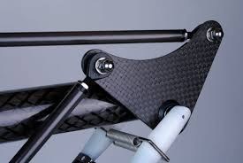
A composite is a mixture of materials, where some of the materials provide tensile strength and others provide compressive strength. To put it more clearly, picture a concrete column: in that column, steel rebar provides tensile strength while the concrete provides compressive strength. The same equation holds in composites, except the scale is far finer. In composites, resin provides compressive strength, while the fibers embedded in the composite provide tensile strength. Even though composite parts offer remarkably good properties, building robots entirely out of composite is beyond most robot builders' reach. In some cases, though, such as building a robot's body shell, the manufacturing process is easier, and with less than an hour of study and a bit of guidance from composite-parts manufacturers, you'll be able to make them yourself. This section of the book is written with building a robot's body shell in mind. Generally, the manufacturing process follows one of two approaches, depending on the number and precision of parts needed:
If high precision is needed, if the number of parts exceeds three, or if the part's external dimensions matter, a model of the part is built first. The model can be made from wood, polyamide, or any other material - though it's worth noting that the model must have no sharp corners and its surface must be polished smooth. There are other key considerations too, which don't apply universally to every part, so it's best to consult composite-parts manufacturers to identify them before building the model. Once the model is built, it's handed over to fiberglass fabricators to take a mold off it. In this process, the model is coated with a release agent and wax, then a mold is formed over it using materials such as fiberglass. Once the mold has cured, its inner surface is coated with a release agent, and a composite layer - which might be carbon fiber, fiberglass, or Kevlar - is laid into it. Once laid in place, the fabric is soaked with resin using a brush; the next layer of fabric is then placed over the previous one and likewise soaked with epoxy resin. This layering process continues until the part reaches the desired thickness. The part is then left to cure, after which it's removed from the mold, and the process repeats for subsequent parts. If you want to produce a very small number of a given part, where the internal dimensions matter but the external dimensions aren't especially important, you repeat the previous process - except this time, no mold is taken from the model; the layering process is applied directly onto the model itself. In other words, instead of building inside a mold, the manufacturing happens on the polished model directly. In some jobs, manufacturing is done using several mold sections, with each part of a complex piece built using its own separate mold - two-piece molds being the most common. Given how specialized and extensive this topic is, we won't go into further detail here. Parts made this way are vulnerable to sunlight and heat exposure, so only expose them to direct sunlight when absolutely necessary. If prolonged sun exposure is unavoidable, use light-colored paint on the part and increase its thickness. In some applications, such as flight components, you don't need to worry about sun exposure, since the parts are cooled by airflow. Parts made using the second method tend to have a rough exterior finish and may show some distortion. To achieve a good finish, you can turn to auto body shops, which use sanding and body filler to smooth the surface and paint it however you like. It's best to choose your color from the common range of automotive body paints. Before sending the part off for bodywork, make sure all necessary holes are drilled into it first, since drilling after filling and painting can chip away a large section of the paint. Thicker parts are more durable but heavier; thinner parts are lighter but offer weaker strength characteristics, and removing them from the mold is difficult and can damage them in the process. Generally, three composite materials are used in layering - fiberglass, carbon fiber, and Kevlar - listed here in order of how common, and how expensive, each one is. The sample part shown is made of fiberglass with a thickness of about 0.25 millimeters. The authors reinforced high-stress areas of the part using carbon fiber tape. Fiberglass is made from glass fibers, and its fabric is easy to find in whatever thickness you need; it's also more affordable than the other fabrics. Parts made from carbon fiber offer higher mechanical strength, letting you build lightweight, highly durable parts. Carbon-fiber fabric conducts electricity, so it acts as a barrier against radio waves and shields them - something to keep in mind during design, since a body shell made this way could disable a communications system and, with a bit of bad luck, significantly reduce its effective range. That said, this is a double-edged sword, since such a body shell can also block radio interference - using this material correctly can actually work in your favor.
Kevlar (Aramid Fiber)
This is another type of fabric with extremely high tensile and shear strength. Specialized mountaineering ropes and bulletproof vests are made from this material. If you need a part or component that resists explosions, shrapnel, or bullets, this material is the best option. Sourcing raw Kevlar and manufacturing parts from it comes with a lot of difficulty. To start with, because this material has military applications, buying it online is difficult. Some individuals and domestic companies do supply this fabric, but their stock and range of options are quite limited. Unlike fiberglass and carbon fiber, Kevlar fabric can't be cut with ordinary scissors - it needs special shears, which have to be sourced from abroad. After building composite parts, it's usually necessary to cut and drill them further. This is difficult on aramid/Kevlar composites, because the fiber's high tensile strength causes it to catch on the drill bit and wind around it, leaving a hole quality that leaves the builder unhappy. Glass, carbon, and Kevlar fabrics come in various thicknesses, specified in grams in the fabric catalog. Weave patterns also vary widely - some fabrics have strength in one specific direction, while others have strength in two or more directions. Some fabrics even combine several fiber types in their weave - for example, using fiberglass fiber in one direction and carbon fiber in another.
Some builders want to produce strong parts using cheap materials like fiberglass. To do this, you can reinforce certain areas of the part with thin fabric strips, tape, or even carbon-fiber or Kevlar threads. For building composite parts, you can turn to two groups of specialists: the first is model-airplane builders, who can produce very lightweight, strong, precise parts - though their working style and the value of their time and expertise tend to drive up the final cost. The other group is manufacturers of fiberglass automotive bumpers; these shops generally use a mix of cheap resins and glass fiber. The final cost with this method is very low, but the quality isn't great. If you'd like to get some hands-on experience with fiberglass, you can go to a pharmacy and buy lightweight orthopedic casting material. This "light cast" material is used in orthopedics and is essentially a fiberglass fabric soaked in resin that hardens on first contact with water, becoming water-resistant once cured. These casting materials are only recommended for a first hands-on experiment, since many of them have less-than-ideal properties. You can drill composite parts using ordinary drill bits or a mini drill at low speed. To cut composite parts, use a mini drill fitted with new, sharp bits. To do this, mount a small bit in the mini drill, mark a line at the cut location, lay a metal straightedge along the line, and clamp it in place with one or two locking pliers. Then position the bit against the part, keep its edge running flush against the straightedge, turn on the drill, and create a large number of closely spaced holes along the cutting path. Once you've finished drilling, run the bit back through the holes along the straightedge so the holes connect into a continuous, straight cut. This process takes a great deal of time and patience - I remember one night I stayed up until morning just to cut a limited number of pieces to the quality I wanted. Another way to cut composites is using a tool called an acrylic (Plexiglas) cutter, available at architectural-supply stores.
Drilling Holes
The drilling process barely needs explaining. Generally speaking, it's done using a drill: the bit's two sharp cutting edges shave material off the workpiece's surface, and the shavings are cleared away through the flutes on the bit.
Drills come in an enormous variety, and using three particular types is unavoidable in robotics. A fourth type is introduced here just for general knowledge. Here's how each works:
Hand Drill
This drill is portable and sees the most use of all - when needed, it can stand in for a mini drill or a pillar drill, and it's an essential, inseparable part of any toolbox. These drills run at high speed and power; it's best not to run them continuously for long stretches. That said, industrial-grade drills, such as blue Bosch drills or Hilti drills, don't need this precaution.
At the point where the handle meets the body sits the on/off trigger, and close to it is a lock button. If you want the drill to run continuously, you press this button in. The rotation speed of these drills can be adjusted up or down with a button, and they're generally two-speed. The lower speed gives higher precision and puts less strain on the drill. Some drills have a variable trigger, letting you control speed based on how hard you squeeze it. Some drills have a button labeled "hammer," suited to construction work, which can actually damage precision work - make sure it's switched off before starting a precision job. The bit is secured in a part called a chuck, tightened in place by hand along with a special chuck key. Make sure that once it's switched on, the bit doesn't wobble; if it does, either the bit is dirty, it isn't seated properly in the chuck, or the chuck itself is damaged. Any of these issues needs to be fixed before doing precision work.
Drills come with an extra handle that attaches near the chuck end, which helps with more precise control - you should use it, for example, when working with long bits. Drills also have special stands: mounting the drill on one of these stands lets you drill precise, vertical holes. You can even use them for minor milling-like tasks, such as flattening a surface. Another useful task made possible this way is drilling to a precise depth. Inside the drill is a powerful fan that cools it; the air it blows out is strong enough that you can also use it for blowing away debris and cleaning. Some portable drills have a battery in the base - these have lower output power, but since there's no cord, drilling with them is more convenient, and they can be used anywhere. When drilling, keep the bit and the hole cool.
Pillar (Bench/Workshop) Drill
This drill has a table that the workpiece is clamped to, and a lever lets you lower the drill assembly slowly and with light force until the bit engages the workpiece. Most of these drills run on three-phase power and are quite powerful. If the workpiece gets stuck or welds itself to the bit, the drill doesn't stall - instead, the workpiece starts spinning. These drills run at low speed, which generates less heat at the workpiece and lets the work proceed with greater precision. At the top of the drill is a housing with two multi-step pulleys and a rubber belt; shifting the belt between pulley steps lets you raise or lower the drill's speed. For drilling hard or gummy metals like titanium and stainless steel, use very low speeds. Always unplug the drill before changing its speed setting, to avoid accidents.
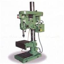
Some pillar drills rotate the bit in one direction as it descends, and reverse its direction as it retracts. These drills speed up tapping and improve its precision. A special tap, called a machine tap, is mounted on these drills. You can find this type of drill at automatic-lathe (screw-machine) workshops.
Mini Drill
These are small drills typically used for drilling electronic circuit boards, precision hole-making, precise wire cutting, and precision grinding. They run at high speed. There are two types: the first has no motor of its own and is connected via a flexible shaft to a hand drill, drawing its power from it. These have high power, but the attached flex-shaft makes them awkward to work with; they also vibrate quite a bit, so overall we don't recommend them. The other type has its own small DC motor, powered through an adapter. These drills are sold in boxed kits with accessories, at prices ranging from roughly 3,000 to 90,000 tomans. This type has two buttons - one for turning the drill on and off, and another for locking the shaft in place when swapping out bits. Typically, the largest bit that fits this drill is 3 millimeters.
Radial Drill
In appearance, this resembles a pillar drill, except much larger. This drill can work very precisely, and because of its precise axial motion, it can also handle some basic milling operations. All drill bits suited to metal and plastic are made from steel alloys and appear black or gold in color, marked HSS. For very hard, gummy metals like stainless steel, spring steel, and titanium, the best-suited bit is HSS-Co, which incorporates cobalt in its composition and comes in brown, red, or silver - priced at roughly ten times an ordinary bit. Bits containing titanium or diamond also exist on the market, but in most applications, cobalt bits make them unnecessary. Certain bit sizes are considered specialty items - for instance, a 1/2 mm bit is a specialty size that might cost three times as much as a 2 mm bit. Once a bit goes dull, you can sharpen it using a rotary grinding wheel; learn this skill from machinists. A spinning drill bit can pierce skin far faster than you'd expect - to this day, two bits have gone through the author's own hand, and it's an ever-present risk. If a bit does go through your hand, get to a doctor immediately, since injuries like fractures, severed nerves, severed tendons, and infections can result. Make sure, after tightening the bit, that the chuck key isn't left in the chuck - if the drill starts up with the key still inserted, it flies off and becomes a serious hazard.
Shaper (Shaping Machine)
On this machine, the tool moves along a straight line while the workpiece stays fixed. The cutting tool attaches to a tool holder mounted on the machine's ram, which moves back and forth. On most machines, cutting happens as the tool moves forward; on some machines, it happens on the return stroke instead. A handle at the top of the machine lets you lower the tool precisely to take a cut. The table under the workpiece has one degree of freedom and can be moved along a single axis. The tools used on this machine resemble those used on a lathe, though they differ in size and how they're ground. Shaping machines are used to cut grooves, slots, keyways, and similar features. In building robots, our main use for this machine is cutting keyways inside gear bores. A special variant called a planer (gate-type shaper) is used for machining very large parts and has no application in robotics.
Automatic Bar Turning (Screw-Machine Work)
Common automatic-turning machines have a structure similar to a regular lathe. In these machines, a length of metal stock - which might be round bar or a shape like hexagonal stock - is loaded into the machine. Inside, several tools take turns machining the bar at high speed, and the finished part is parted off from the bar. The bar then advances slightly and locks in place, the operations run again, and the process repeats. With this method, you can bore holes into parts, turn contoured outer surfaces, and produce some genuinely interesting parts. These machines can produce parts accurate to five thousandths of a millimeter. This method suits producing small parts and can churn out large quantities cheaply. Whenever you need a large number of small turned parts, it's worth consulting an automatic-lathe shop. With this method, the cost of even the most complex parts usually comes to less than 500 rials, unless the quantity is very small - the higher the production volume, the lower the manufacturing cost per part.
In this method, the shop supervisor's skill plays a decisive role in work quality. It's best to entrust the job to experienced, seasoned workers - especially those who genuinely enjoy this kind of work. Small parts are easy to lose, so it's best to produce somewhat more than you actually need.
Modeling, Mold-Making, and Casting
Melting metal and pouring it into a container called a mold is known as casting. This technology encompasses a wide range of methods, including powder metallurgy, forging, sand-mold casting, and others.
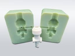
Casting has limited application in prototype-stage robot part production, and you'll likely have no need for it in prototype work. The only casting method the authors of this book have used so far in prototype robot-part production is sand-mold casting. In building robot parts, we turn to this method when a part would generate a lot of machining waste and require a lot of machining time, and when we need a significant quantity of that part.
To cast a part, a model of it is built first. This model might be made of wood, plastic, plaster, or metal, but most model-making shops build it out of wood. It's painted to extend its life and reduce how much sand sticks to it. Depending on the material to be cast and the post-casting operations involved, standard paint colors are applied to the model. This wooden model is called the "master pattern." The model's surfaces are given a slight draft angle so it releases easily from the mold.
Casting is done inside special sand containers called flasks. These consist of two boxes - the cope and the drag - each completely open on top and bottom, designed to sit on top of each other and lock together. Foundry sand is a mixture of sand, a refractory binder, and water, giving it the appearance of slightly damp sand. In the casting process, the pattern is first placed on a table and dusted with a parting compound so the sand doesn't stick to it. The drag is then placed around the pattern and filled with sand, which is packed down evenly using a tool called a rammer. More sand is added and rammed again; after repeating this process several times, the sand's surface is smoothed with a trowel and the assembly is flipped over. If the pattern is a two-piece pattern, the second piece is placed on top; whether the pattern is one piece or several, parting compound is dusted over the pattern's surface and the sand already packed in the drag. The cope is then mounted on the drag, and two thin rods are inserted into it - one positioned away from the part, used as the sprue for pouring metal in, and the other positioned directly above the part, used as a riser for venting gas. Sand is poured in several times and packed down with the rammer. Once finished, the sand surface is smoothed with a trowel and the rods are withdrawn. The two flask halves are separated, and the pattern is carefully removed from both. In the drag, directly below where the molten metal will enter, a small pouring basin is formed, along with a channel (runner/gate) leading from it to the part cavity; at the metal-entry point in the cope, a small funnel-shaped basin is formed as well. The two flask halves are then placed back together, and molten metal is poured into the resulting mold cavity. In casting, holes in a part are formed using a core, made from a special type of sand; to hold cores with tricky shapes in place, thin metal pieces called chaplets are used, made of a metal that melts and dissolves into the poured metal itself. The pattern is oriented for casting so the working surface area is large and the height stays low. The skill and precision of the technician carrying out the work has a direct effect on quality, so choose your foundry carefully and pick workers who genuinely care about the job. In this method, the part shrinks as it cools; to keep this shrinkage from causing problems, the pattern needs to be made larger than the target part. Sand casting works for a wide range of metals, but most commonly it's used with aluminum and cast iron. Aluminum's coefficient of linear expansion between 0 and 100°C is 0.0000238, and its melting point is 659°C. For cast iron, the corresponding figures are 0.0000105 and 1,150-1,200°C.
To bring a part to its target dimensions, it can be machined after casting. For this, machining allowance needs to be planned into the master pattern's dimensions. Because of the metal's weight, the surface facing the bottom of the sand mold - and, as a result, the corresponding part surface - may come out slightly flawed, so machining in these areas is unavoidable. It's recommended to allow 3 millimeters of machining stock on bottom-facing surfaces and 5 millimeters on top-facing surfaces.
The metal's crystalline structure may come out uneven with this method, or tiny bubbles called porosity may form in the part. So this method shouldn't be used for parts that need to withstand high mechanical stress. Foundry costs are calculated based on the weight and type of the material being cast.
Spring Manufacturing
Some shops specialize in supplying springs. Before making a custom spring, it's best to search these shops first and adjust your design slightly to match one of the springs already available - ready-made springs are very inexpensive. If you do need a custom spring, you can easily hand your spring drawing over to a spring maker. Nearly any spring you design can be manufactured, but it's best to consult with a spring maker before finalizing the design. Springs are usually available in several different materials. Stainless-steel springs have a better appearance, and you can be confident their specifications will match your design calculations. Order the spring slightly longer than needed, then shorten it with a grinder after manufacturing. Springs come in many varieties, but based on our experience, three types see the most use in robotics, described below:
Cylindrical Compression Spring
This spring has a cylindrical cross-section and stores energy when compressed.
Cylindrical Extension Spring
This spring has a cylindrical cross-section and stores energy when stretched.
Single-Coil Spring
This spring is a circular ring made from spring alloy and is used in building omnidirectional wheels.
Grinding
There are countless grinding methods and machines, but this process is generally done for three purposes:
- Removing excess metal
- Finishing a metal surface
- Final machining to bring a part to precise dimensions
In most grinding processes, a rotating grinding wheel contacts the workpiece's surface and removes material from it. Never grind aluminum, since it clogs the wheel's pores, and within moments the wheel becomes useless.
Some grinding methods you may need in robotics work are described below:
Surface Grinding
Cylindrical Grinding
This method is used to produce shafts with very precise dimensions. The process is applied to the outer surface of cylindrical parts such as shafts. In cylindrical grinding, the workpiece moves back and forth along its own axis; for large, long parts, the grinding wheel itself moves back and forth instead, a technique called traverse grinding. A cylindrical grinding machine is specified by its maximum workpiece diameter and length. On a universal grinding machine, both the workpiece axis and the wheel axis can pivot in the horizontal plane, letting it grind tapered shafts and similar parts.
Bench Grinder
This is an inexpensive, widely used machine - essentially a double-shaft motor mounted on a special stand, with a grinding wheel, wire wheel, or felt buffing wheel attached to each end. It's used for grinding away excess metal, sharpening bits and tools, and similar tasks. If a wire wheel is attached, you can use it to finish and clean parts - for example, cleaning up a weld joint. If a felt wheel is attached, you can use it for polishing. In machining workshops, two types of wheels are typically mounted on this machine - one for everyday work, and the other for sharpening carbide tools.
Die Grinder
Some grinding stones have a metal core that extends outward as a shank. You can easily mount these onto a drill, or onto a specialized high-speed tool called a die grinder. These stones are used to remove excess material from metal parts. If you coat the stone with grease, you can use it to grind aluminum. That said, only use grease-coated stones on a drill running at low speed, to reduce the risk of the stone shattering and becoming dangerous. Some die-grinder attachments come fitted with sandpaper, felt, or a wire wheel instead of a grinding stone - these are used for cleaning and finishing a work surface.
Painting
Painting serves various purposes, but it's mostly done to prevent rust and corrosion, and to make the robot look attractive and clean. In most cases, large parts such as the body shell go through painting. In the overall process of building machines and robots, the visual quality of the work plays a major role in how a client perceives the polish of the work. This matters so much that an experienced machine-builder once told me: "Five percent of your design and manufacturing effort should go toward making the work look appealing." In every painting process, because of the paint's thickness, a part's dimensions change slightly - so this approach isn't feasible for every part. Keep in mind that all machining and drilling on a part must be complete before the painting process begins. While working on robots, hands stained with solder flux, oil, and grease constantly come into contact with the robot and dirty it; using darker paint colors makes this grime less noticeable. Don't dismiss the psychological effect of color, either - some dark colors, like black or metallic gray, make a robot look more striking and can have a psychological effect on competitors. Some colors, like yellow, are more visible from a distance, while colors like red are harder to spot from far away. Colors like olive green suit military-style work better. For very lightweight projects, painting can be skipped altogether. The robotics projects the authors have been involved in have used three different painting methods, described below:
Powder Coating and Oven Curing
In this process, an electrostatic charge is induced in both the paint and the part, and the paint is sprayed onto the part; afterward, the part is moved into an oven and cured. Equipment for this kind of painting is expensive, and buying it isn't economically justified for robotics work. Many paint shops across industrial areas offer this service. These shops typically choose their color based on their largest orders, running a particular color each day or week, and our job gets folded into whatever bulk order is running at the time. Black and white are usually the most common colors used at these shops, and with a bit of patience, you can time your job to arrive on a day when one of those colors is being run. For aluminum parts, where paint doesn't adhere well to the surface, this method is the best option available, and its cost is reasonable. Once aluminum parts have been painted this way, they can be repainted again using any other method you like.
Automotive Paint
For painting composite and steel body shells, you can take them to an auto body shop to be sanded, filled with body filler, and painted. This method gives you full freedom in choosing your color, including metallic finishes - though metallic paints do have a negative effect on how well radio waves pass through the body shell. The quality of work with this method is higher than the other approaches; the first time we had a robot body painted this way, we could hardly believe how good and appealing the finished result looked. That said, this method costs considerably more than the others.
Spray Painting
This method is quick and cheap. You can pick up a few cans of inexpensive spray paint and use them directly. Use paint colors that are widely available in the market and easy to restock. It's best to spray from a fair distance from the part, and control the spray volume so paint droplets and runs don't form on the surface. To avoid these issues and improve quality, it's recommended to apply several light coats, spraying a small amount of paint each time, rather than one heavy coat.


In this process, paint powder gets drawn directly into the respiratory system, so a cloth mask should be worn, and the process should be carried out outdoors. Doing this indoors leaves paint powder settled on the floor within a radius of several meters.
Steel Bluing (Blackening)
When you bring up blackening with machining specialists, they'll usually describe various steel carburizing processes that harden the steel and change its color. But the blackening process we mean here isn't a heat-treatment or carburizing process. In our blackening process, a finished steel part goes through a treatment that turns the metal's surface black while making it resistant to rust - all without changing the part's dimensions. What's more, the surface of parts treated this way looks attractive, and because it's black, grime such as oil doesn't show up on it.
Argon (TIG) and Silver Welding
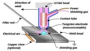
Welding is a method for joining two parts using molten material. This technique dates back to ancient Rome. Welding techniques come in enormous variety, but this section covers argon (TIG) welding and silver brazing, which belong respectively to the electric-arc welding family and the flame-welding family. Both are common methods that you'll certainly be able to find available. In TIG welding, an electric potential difference between the electrode and the workpiece establishes a stable spark, or electric arc. The electrode is made of tungsten and doesn't melt, but the workpiece melts at the point the arc strikes it. To produce more molten material and fill the intended gap, a filler rod made of the same material as the workpiece is fed into the melt. During the process, argon gas flows under pressure from around the electrode into the weld area, isolating the surroundings of the molten metal. This welding method delivers high precision and quality.
After TIG welding, don't cool the part with water - let it cool in ambient air instead, since rapid cooling hardens the part and makes it difficult to machine afterward. Keep in mind that TIG welding penetrates deep into the part. Metals such as aluminum, stainless steel, and titanium weld very well with this method. Silver brazing heats the joint with a flame, then feeds in a filler rod, which melts and joins the two parts together. This method is widely used in eyeglass repair, and providers of this service can be found in most industrial areas. It's suited to welding very small, delicate parts.
Both of these methods are expensive, but their quality justifies the price. In these processes, the welder's skill has a huge effect on the quality of the work. We recommend giving a few similar sample pieces to different welders and, at the cost of a small loss, identifying the most skilled welder in your area. Quality welding is difficult work and belongs to welders who enjoy their craft, have been properly trained, and are sharp-minded - don't hand the job to people who complain about their lives, are undisciplined, low on morale, or lack an active mind. Industrial welding shops, like machine shops, can be found everywhere, and with a bit of asking around at mold shops and machine shops, you can track them down. Don't look directly at the welding arc while it's running, and during TIG welding, keep your distance from the weld site to avoid radiation exposure.
Instant (Drop) Adhesives

A robot's electronics involve a great deal of variety and specialized function, since all mechanical calculations ultimately depend on how efficiently the electronic components perform. Good electronics finish off half the work of building a robot. A robot's electronics are made up of three main sections:
- Power supply
- Sensors
- Microcontroller and ICs
Introduction to Electronic Components
Electric Current
An electrical circuit is a path made up of a power source, electrical components, and conductors. Whenever this path is closed, electrons flow from the power source's negative terminal into the circuit, pass through the electronic components, and enter the battery's positive terminal. The battery acts like a pump, injecting electrons into the circuit. The movement of electrons through a circuit is called electric current. Before electrons were discovered, it was believed that electric current resulted from the movement of positive charges, starting at the positive terminal and returning to the negative terminal after traveling through the circuit. Today, though, we know that in metals, positive charges are stationary and can't move through solids easily, whereas in conductive liquids and gases, both positive and negative particles move. This original convention for current direction has been kept ever since, since what matters about electric current is its nature and magnitude in the circuit, not its direction - and the laws of electricity hold true under this assumption regardless. The unit of current is the ampere (A). When one coulomb of charge (6×10^18 electrons) passes through any point in a circuit each second, the circuit's current is 1 ampere (1 A). Electric current is measured with an ammeter.
Direct and Alternating Current
Direct current (DC) flows in only one direction through a circuit - by convention, from the source's positive terminal toward its negative terminal - and doesn't change for as long as the circuit stays closed. Batteries produce direct current. Alternating current (AC) is current whose direction and magnitude constantly change: the current rises from zero to a peak value in one direction (+), then falls back to zero, before rising again in the opposite direction (−), reaching that same peak magnitude before falling back to zero - and this cycle repeats rapidly.
Frequency of Alternating Current
The frequency (F) of alternating current is the number of complete cycles it completes in one second, measured in hertz (Hz). The AC frequency supplied by electrical grids in most countries around the world is 50 Hz.
Voltage (Potential Difference)
Electric potential, usually denoted V, is the amount of electrical energy per unit charge, measured in volts. It's usually discussed as the potential difference between two points. By definition, a potential difference of one volt between two points means that one joule of work is required to move one coulomb of positive charge from point "A" to point "B."
Electrical Resistance
Electrical resistance, or impedance, describes how strongly a physical object resists
the flow of electric current through it. The SI unit of electrical resistance is the ohm. The resistance of any conductor in a circuit is denoted R and determined by the equation below, where V is the potential difference across the conductor in volts and I is the current flowing through it in amps. This equation is known as Ohm's law, and its meaning is stated as follows: at a constant temperature, the current flowing through a conductor is proportional to the potential difference across it.
Resistor Characteristics
The resistance value, expressed in ohms. The power rating is the maximum dissipated power the resistor can tolerate, given as follows:
Tolerance (or precision) is the maximum permitted deviation of the resistance value from its stated value (expressed as a percentage).
Determining Fixed Resistor Values
Color Codes
For this type of resistor, colored bands indicate the resistance value. The first color band always sits closer to one end of the resistor. The resistance value is calculated using the formula below:
In this formula, the first and second color bands (and the third, for 5- and 6-band resistors) determine the value A. The third band (the fourth, for 5- and 6-band resistors) determines the value B. The fourth band (the fifth, for 5- and 6-band resistors) indicates the error percentage, or tolerance (value C). The sixth band indicates how the resistance changes per unit change in temperature (the temperature coefficient).
Printed Codes
The code printed on a resistor combines letters and digits. R means ×1, K means ×10^3, and M means ×10^6. The position of the letter also marks where the decimal point falls in the resistance value. Each resistor's tolerance is indicated by adding a letter - J = 5%, K = 10%, M = 20% - to the symbols and digits. For example, "5K6K" denotes a resistance of 5.6 kΩ ± 10%.
Resistors aren't manufactured in every possible value - only certain specific values are available. Other values can be obtained by combining resistors in series and parallel. The standard E24 resistor values are as follows:
Variable Resistors
A variable resistor is a type of resistor whose resistance can be adjusted from zero up to its maximum value. As shown in the figure below, this component has three terminals: the maximum resistance sits between points A and B, and the resistance from point C to either of these terminals can be adjusted by turning the wiper.
Variable resistors come in several types. The most common type is the potentiometer. Potentiometers are single-turn devices with a maximum power rating of 2 W. Their resistive track can be made from carbon or cermet (a mixture of metal oxide and aluminum), but for power ratings above 2 W, a wire-wound type is used instead. Another type of variable resistor is the multi-turn potentiometer, whose wiper can rotate through several full turns. Multi-turn potentiometers are used where precise adjustment and low power are needed. The high-power type of variable resistor is the rheostat ("volume" type).
Resistors in Series
A series connection means two or more resistors are connected one after another with no intervening component between them. In a series connection, the total resistance equals the sum of the individual resistances. In a series connection, the total resistance is greater than any single resistor in the chain.
Resistors in Parallel
A parallel connection means both ends of two or more resistors are connected directly to each other. In this case, the total resistance is smaller than any individual resistor and is found using the following relationship:
Voltage Divider
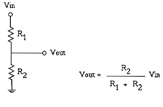
When two variable or fixed resistors are connected in series, as shown in the figure, the voltage between them is given by the relationship below. This principle is used in a potentiometer to produce a variable voltage. When 5 volts is applied across a potentiometer's two outer terminals, adjusting the potentiometer lets you draw a variable voltage between zero and five volts from its middle terminal.
Capacitor
A capacitor is an electrical component that can store electrical energy as electric charge. Various types of capacitors are used in electrical circuits. A capacitor is denoted by the letter C, from the word "Capacitor."
Capacitor Construction
A capacitor's internal structure consists of two main parts:
a. Conductive plates
b. Insulation between the conductors (the dielectric)
Whenever two conductors face each other with an insulator placed between them, a capacitor is formed. A capacitor's conductive plates are typically made of aluminum, zinc, or silver with a fairly large surface area, and the insulator (dielectric) between them can be air, paper, mica, plastic, ceramic, aluminum oxide, or tantalum oxide. The larger a material's dielectric constant, the better its insulating properties. For example, air has a dielectric constant of 1, while aluminum oxide has a dielectric constant of 7 - meaning aluminum oxide's insulating property is seven times that of air.
Flat (Parallel-Plate) Capacitor
Two parallel metal plates with an insulator called a dielectric between them (such as air or glass). Connecting the capacitor's plates to a power source charges the capacitor; the potential difference across the capacitor's plates will equal the potential difference across the source.
Capacitance (C)
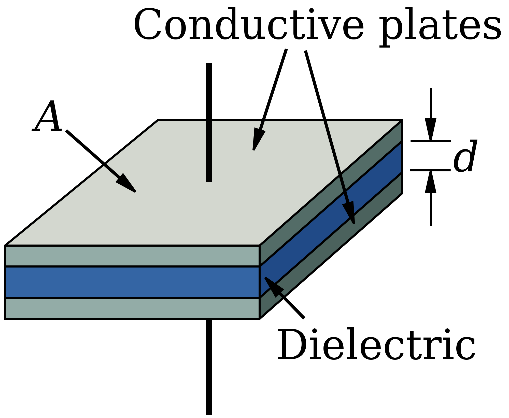
Capacitance is the ratio of the charge accumulated on the plates to the potential difference across the battery's terminals - a constant value.
C=kε0A/d
Capacitance, in farads = C
Stored charge, in coulombs = Q
Potential difference across the source, in volts = V
ε0 = the permittivity of free space, equal to:
K (unitless) = the dielectric constant, which differs for each material. For air and vacuum, K is approximately 1.
A = the capacitor's plate area, in m²
D = the distance between the two plates, in m
One farad is a very large unit and denotes a high capacitance. So smaller units are also commonly used for capacitors: the microfarad (μF), nanofarad (nF), and picofarad (pF) are the smaller units of the farad.
A Few Notes
Experiments show that a capacitor's capacitance doesn't depend on the amount of charge (q) or the potential difference across it (V) individually, but on the ratio q/V.
The electric charge stored in a capacitor is directly proportional to the potential difference across it. Capacitance is inversely proportional to the distance between the two plates.
Capacitance is directly proportional to the area of each plate and to the dielectric material (K).
Charging a Capacitor
When an uncharged capacitor is connected across a battery, electrons start flowing through the circuit. As a result, one plate takes on a positive charge and the other a negative charge - the plate connected to the battery's positive terminal becomes positively charged, and the other becomes negatively charged. The capacitor is "charged" once it has stored a certain amount of electric charge - meaning that even though the switch stays closed, no current flows through the circuit anymore, and the current effectively drops to zero. In other words, the moment an uncharged, empty capacitor is connected to a source in a circuit, the ammeter needle returns to zero again after a short while - meaning no more current passes through the circuit. At this point, we say the capacitor is fully charged.
Discharging a Capacitor
Consider a capacitor that starts out fully charged. We connect its two terminals together with a wire. In this state, current flows briefly through the circuit, continuing for as long as charge remains on the capacitor's plates. After a while, the current drops to zero - meaning no more charge remains on the plates, and the capacitor is now discharged. If a capacitor is fully charged, no current will flow; if it's fully discharged, current won't flow either.
Connecting Capacitors
Capacitors are connected in a circuit in one of two ways:
- Parallel
- Series
Connecting Capacitors in Parallel
In a parallel connection, capacitors share two common points. In this configuration, the potential difference is the same across all the capacitors. The total charge stored in the circuit equals the sum of the charges stored in each individual capacitor.
Equivalent Capacitance in Parallel:
When several capacitors are connected in parallel, the equivalent capacitance equals the sum of their individual capacitances.
Connecting Capacitors in Series
In a series connection, capacitors share only one common point, and only the two outermost plates of the chain connect to the source and receive charge directly from it. The facing plates receive their charge through electrostatic induction. As a result, the amount of charge on every capacitor in this configuration is equal.
- The potential difference across the whole circuit equals the sum of the potential differences across each individual capacitor.
- The total capacitance in a series configuration - the reciprocal of the equivalent capacitance - equals the sum of the reciprocals of each individual capacitance.
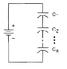
Equivalent Capacitance in Series:
Capacitor Applications
Since capacitors store electric charge, they can be used to create uniform electric fields. Capacitors can hold electric fields within a small volume, and they can also be used to store energy. Capacitors are likewise used to smooth out fluctuations in a DC voltage level. They're also used as filters in circuits, since capacitors readily pass AC (alternating) signals while blocking DC (direct) signals. Together with resistors, capacitors are used in timing circuits. A capacitor is essential to the correct operation of nearly every electronic circuit.
Capacitor Applications in Digital and Analog Circuits
In digital circuits, capacitors are used as energy-storage elements that charge at one moment and discharge at another. In analog circuits, though, a capacitor is used to isolate a DC source from an AC source. A capacitor behaves like a short circuit toward AC voltage, letting it pass in or out, but behaves like a barrier toward DC voltage, blocking it from entering or leaving the isolated portion of the circuit.
Types of Capacitors
Capacitors come in many types and differ from one another in shape and size. Some capacitors are oil-filled and quite bulky, while others are tiny - no bigger than a lentil.
Fixed Capacitors
These capacitors have a set capacitance that doesn't change under normal conditions. Fixed capacitors are classified and named according to the dielectric material used in them, and are used for various purposes. These include ceramic, mica, film (paper and plastic), electrolytic, oil-filled, gas-filled, and a special film type. If the dielectric material forms through a chemical process, the capacitor is called an electrolytic capacitor; otherwise, it's called a dry capacitor. Oil-filled and gas-filled capacitors are mostly used in the power industry, in electrical circuits for starting equipment or correcting power factor. The remaining fixed capacitors each have their own particular characteristics.
Variable Capacitors
Generally, a capacitor's capacitance can be changed by adjusting three factors: the distance between the plates, the plate area, and the dielectric type. Variable capacitors work by changing the overlapping area of the plates, or by changing the dielectric's thickness. Capacitance is directly proportional to the overlapping area of the two plates. Variable capacitors are generally of the air-insulated or plastic-insulated type. The type adjusted via a movable shaft is called a "variable" (tuning capacitor), while the type adjusted with a screwdriver is called a "trimmer." Variable capacitors range from 10 to 400 picofarads, while trimmer capacitors range from 5 to 30 picofarads. These capacitors are used in radio receivers to tune in a station's frequency.
These capacitors are used in radio tuning circuits, which is why they're sometimes called "tuning capacitors." Their capacitance is quite low, around 100 to 500 picofarads, and because of this low capacitance, they aren't used in timing circuits. Timing circuits use fixed capacitors instead, and if the period needs to be adjusted, this is done using a resistor.
Trimmer Capacitors
Trimmer capacitors are small variable capacitors with a very low capacitance, ranging from about 1 to 100 picofarads, and are mostly used in the tuners of high-frequency circuits.
Ceramic Capacitors
The ceramic capacitor is the most common non-electrolytic capacitor, using ceramic as its dielectric. Ceramic has a high dielectric constant, which makes it possible to build high-capacitance capacitors in a small size compared with other types - and, as a result, they can handle a high working voltage. Ceramic capacitors typically range from 5 picofarads to 0.1 microfarads in capacitance. This type is manufactured in disc and cylindrical forms, and ceramic capacitors work at frequencies above 100 MHz. Their major drawback is that their capacitance depends on ambient temperature, since capacitance shifts as temperature changes. This capacitor is used in electronic circuits such as communications and radio-frequency circuits.
Film (Sheet) Capacitors
Film capacitors use paper or plastic materials as the dielectric, thanks to their flexibility. This group of capacitors is built in two forms:
Paper Capacitors
This type's dielectric consists of a thin sheet of porous paper impregnated with a suitable dielectric fluid to keep it from absorbing moisture. To prevent the dielectric fluid inside the paper from evaporating, the capacitor is enclosed in a sturdy, impermeable casing. Because of their dielectric's low dielectric constant, paper capacitors have large physical dimensions - though their advantage is that they can be used at high voltages and currents.
Plastic Capacitors
This type uses thin plastic sheets as the dielectric. The plastic sheets, together with thin metal (aluminum) foil, are rolled up into a tube shape and packaged inside a plastic casing. Today, these capacitors see wide use in circuits thanks to their good characteristics. They aren't very sensitive to temperature changes, which is why they're used in circuits that need stable capacitance under heat. One of the dielectric materials used in these capacitors is polystyrene, which is why they're also called "polyester" capacitors - among the most common types of plastic capacitors. The maximum operating frequency of plastic capacitors is around one megahertz.
Mica Capacitors
This type uses thin mica sheets between the capacitor's plates (aluminum foil), with the whole assembly enclosed in a casing at the end to protect it from moisture. Mica capacitors range from about 0.01 to 1 microfarad in capacitance. Their key characteristics include a high working voltage, long service life, and suitability for high-frequency circuits.
Electrolytic Capacitors
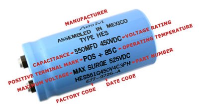
These capacitors are typically in the microfarad range. Electrolytic capacitors are still fixed capacitors, but their size and capacitance are larger than ordinary fixed capacitors. They're also known as "chemical" capacitors - a name that comes from the fact that their dielectric is treated with certain chemical substances that act, in effect, as a catalyst and boost the capacitor's capacitance. Unlike disc-type capacitors, these have positive and negative terminals. A "−" symbol is printed on the body next to the negative lead. The actual capacitance value and maximum voltage rating are also printed on the body. Electrolytic capacitors are made in two types: aluminum and tantalum.
Aluminum Capacitors
Like film capacitors, this type consists of two aluminum foils. One of these foils, on which an oxide layer is formed, is called the "anode," while the other aluminum foil serves as the "cathode." Its internal structure is built by rolling the two aluminum foils together with two layers of porous paper between them, with lead wires attached to the ends of the foils. After rolling, the assembly is soaked in a suitable electrolyte that speeds up formation of the oxide layer, until the two porous paper layers are saturated with electrolyte. The whole assembly is then placed inside a metal casing, sealed with a plastic grommet through which the capacitor's leads pass.
Tantalum Capacitors
This type uses tantalum metal instead of aluminum. Because tantalum oxide's dielectric constant is much higher than aluminum oxide's (roughly three times higher), tantalum capacitors achieve a higher capacitance than aluminum capacitors of the same volume.
The advantages of tantalum capacitors over aluminum ones are as follows:
- Smaller size
- Lower leakage current
- Longer service life
Among the drawbacks of this type compared with aluminum capacitors are:
- Tantalum capacitors are more expensive.
- They're more sensitive to voltage exceeding their rated limit, as well as to reverse polarity.
- They can't tolerate high charge and discharge currents.
- Tantalum capacitors have a capacitance limit (manufactured up to a maximum of 330 microfarads).
Switches
An electromechanical component that opens and closes the path of electric current. Switches are, in effect, metal contacts that separate or connect to interrupt or complete a circuit's current. A switch's behavior depends on the following factors:
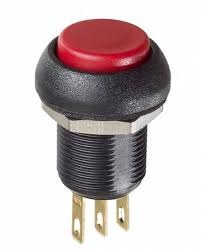
First, the maximum current it can handle, and second, its rated working voltage. These two parameters differ for each switch depending on whether it's used with DC or AC. For example, if a switch's AC working voltage is 240V with a maximum allowed current of 1.5A, these figures might change to 20V and 3A under DC. If such a switch is placed in a circuit that exceeds these ratings, its service life shortens. The factors that shorten a switch's life include the heat generated by current flow while it's closed, and the erosion of its metal contacts while it's open, caused by arcing across the air gap between the switch's two contacts - this arcing is typically worse under DC than AC, since AC current passes through zero twice every full cycle.
Diodes
A diode is an electronic component made from a junction of P-type and N-type semiconductor material. Diodes let electric current pass through in one direction while offering high resistance to current in the other direction.
At the P-N semiconductor junction inside a diode, free electrons and holes cross the junction and combine with each other, forming a barrier, or insulating, layer. A depletion region forms at the junction, containing no free electrons or holes - though atoms that have lost or gained an electron remain on either side of the barrier layer, within the depletion region.
These ionized atoms create a potential barrier, which is about 0.2 volts for germanium semiconductors and about 0.6 volts for silicon semiconductors.
The potential barrier that forms prevents further movement and recombination of electrons and holes across the barrier layer. The P-type semiconductor crystal carries a positive charge, while the N-type semiconductor crystal carries a negative charge.
Diode Biasing
Applying a voltage to a diode is called biasing the diode.
Forward Bias
If the P-type semiconductor is connected to the battery's positive terminal and the N-type semiconductor to its negative terminal, and the voltage exceeds the diode's barrier potential, current will flow in the circuit.
Reverse Bias
If the battery's positive terminal is connected to the N-type semiconductor and its negative terminal to the P-type semiconductor, no current will flow in the circuit.
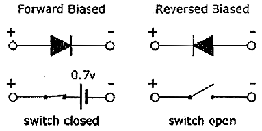
Electrically speaking, a diode allows current to pass once you prepare it by applying voltage in the correct direction (+ to the anode, − to the cathode). The voltage at which the diode begins conducting current is called the threshold voltage, or forward voltage drop, which is roughly 0.6 to 0.7 volts. But when you apply reverse voltage to the diode (+ to the cathode, − to the anode), no current passes through it, aside from a very small current known as leakage current, typically on the order of a few μA or even less. This current is usually negligible in most electronic circuits and doesn't affect the behavior of other components in the circuit.
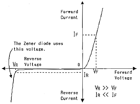
One important point, though, is that every diode has a threshold for maximum reverse voltage - exceed it, and the diode burns out and starts conducting current in the reverse direction too. This threshold is called the breakdown voltage. Diodes are broadly classified into three main categories: signal diodes, used for detection in radios, which carry currents on the order of milliamps; rectifier diodes, used to rectify alternating current and capable of carrying large currents; and finally, Zener diodes, used for voltage regulation. An ohmmeter is used to identify a diode's positive and negative sides, based on how the meter's needle responds.
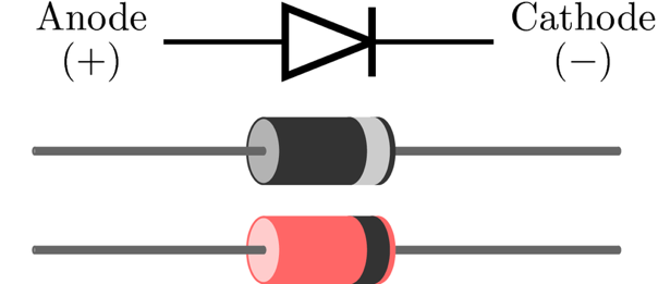
Types of Diodes
- Zener Diode
- Light-Emitting Diode (LED)
- Photodiode
- Zener Diode
A Zener diode, like an ordinary diode, is made from two P and N semiconductor layers. If you connect an ordinary diode in reverse bias and keep increasing the reverse voltage, at a certain voltage the diode will start conducting in reverse bias too. The voltage at which the diode starts conducting under reverse bias is known as the Zener voltage, and by adjusting the doping level, the breakdown voltage of the junction can be controlled.
Zener Voltage: the voltage at which a Zener diode becomes conductive under reverse bias is known as the Zener voltage. Zener diodes are, in effect, a special type of silicon diode, designed so they can sustain a reverse breakdown voltage continuously. There are various families of Zener diodes, depending on their general characteristics, package type, and power rating. Their breakdown voltages align with the preferred E12 and E24 number series (ranging from 2.7 volts to 86 volts).
Light-Emitting Diode (LED)
This diode consists of two types of P and N semiconductor. Whenever this diode is forward-biased with sufficient current, it emits light. The light is generated at the junction between the two semiconductor layers, and the color produced depends on the semiconductor material used.
This type of lamp offers several advantages over conventional lamps, including:
Small size and low space requirements
Durability and long service life (around one hundred thousand hours of operation)
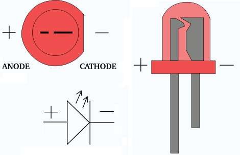
Fast on/off switching of light
Low heat loss
Low working voltage, between 1.7 and 3.3 volts
Low current - a few milliamps - for visible light
Low power, around 10 to 150 milliwatts
Photodiodes
This diode is made from two P and N semiconductor layers, except that the P-N junction, where light shines onto it, isn't covered in black plastic - instead, it's covered with glass or clear plastic so light can reach it easily. Most photodiodes have a tiny lens mounted on top to focus the incoming light and direct it onto the junction.
Transistors
Transistors are among the most widely used components in electronics. They're made in a wide range of models for different applications. One use of a transistor is as an on/off switch; another important use is as an amplifier. From the small transistors used to drive tiny toy motors, to the transistors that control a model-train's motor circuit, they all share roughly the same structure and operating principle, though they're built in different sizes and using different methods. Put simply, a transistor's function can be thought of as current amplification. Consider a small logic circuit that, under certain conditions, produces a very small current at its output - using a transistor, you can amplify that current and then use the stronger current to switch a relay on and off. There are also many cases where you use a transistor to amplify voltage. Naturally, this trait comes directly from the device's current-amplification property: you simply need to pass the amplified input and output current through a resistor to turn a small input voltage into an amplified output voltage. Like diodes, transistors are built from combinations of semiconductor materials. Broadly speaking, semiconductor materials fall into two categories, P and N. A diode uses only these two materials, P and N. Structurally, a transistor can be modeled as two diodes. A transistor uses two P-type materials at different doping concentrations along with one N-type material - these are called PNP transistors. Transistors are also built as NPN. These transistors are shown using the symbol below.
Each semiconductor layer in a transistor has a corresponding lead that connects it to the outside circuit. These leads are called the base, the collector, and the emitter. If you look closely at a transistor's layered structure, there doesn't appear to be much difference between the collector and the emitter - but that's not actually the case, since the collector layer is considerably thicker and larger than the emitter layer, which in practice makes these two layers different from each other despite sharing the same polarity. Even so, diagrams typically show these two layers as identical, for simplicity.
In most cases, we use NPN transistors, so from here on we'll limit our discussion to this type - though everything here can easily be extended to PNP transistors as well. It's a simple task, and you can do it yourself once you're familiar with NPN transistors. In NPN transistors, current flows from the collector to the emitter (in PNP, from the emitter to the collector - always following the direction of the arrow). This current only flows from collector to emitter if:
- The collector voltage is higher than the emitter voltage.
- The base voltage is 700 mV higher than the emitter voltage.
The base current is very small, while the emitter and collector currents are quite large - roughly 100 to 200 times the base current. In fact, the larger the base current, the larger the emitter current becomes too; this is one of the transistor's amplifying properties. Without going into a detailed examination of exactly how a transistor works, we want to introduce you to the simplest circuit you can build with a single transistor, and explain its application. Take a look at the figure below.
We placed separate power sources between E and C, and between E and B. The resistors placed along the path of each of these voltage sources are there purely to limit current, and nothing else - without them, the junctions would burn out from excessive current draw.
Here's how a transistor works: if you forward-bias the B-E junction (bias meaning applying voltage to stimulate the junction) so that this P-N junction turns on - which just takes applying about 0.6 to 0.7 volts across it, depending on the transistor type - then a very large current can be drawn through the circuit formed between E and C. Normally, there's no closed circuit between E and C at all, but the moment you forward-bias the B-E junction, it behaves almost like a short circuit, and you can effectively draw a significant current through the E and C leads. So you can see that establishing a small current IB lets you produce a large current IC. This circuit is the basis of electronic switches in electronic circuits.
Problem:
In a circuit, a current of 10 milliamps flows through the base, and the transistor is built with a gain (hFE) of 120. What current will flow through the collector?
Solution:
Since the gain is 120, the current through the collector will be 120 times the base current. Suppose that 10 mA current came from a microphone, and you connected it directly, through a wire, to a speaker - in that case, the sound coming from the speaker would be very quiet. But if you use a transistor, you'll hear a much louder sound.
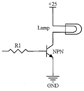
Another use of a transistor is as a switch. Consider a small IC, and suppose the maximum current it can supply is 25 milliamps at 5 volts, and suppose you want to turn on a lamp rated at 25 volts and 500 milliamps. This can easily be done with a transistor, using the circuit shown. When the IC's output is at zero volts, since the emitter voltage is also at ground, or zero volts, the transistor stays off (because the base voltage isn't higher than the emitter voltage - they're equal, both at zero). As a result, no current flows through the transistor, and therefore none through the lamp either. But when the IC's output reaches 5 volts, the transistor turns on, and, depending on the base current and the transistor's gain, current flows through the lamp and lights it. The size of this current depends on resistor R1: the larger this resistor, the smaller the current, and if the resistance is too low, too much current will flow through the lamp, burning out both the lamp and the transistor. You can control the lamp's brightness by replacing R1 with a potentiometer (variable resistor). If this resistor were placed directly in the lamp's own current path instead, a large current would flow through it, which would waste a lot of energy and could even overheat and burn out the resistor itself.
Transistor Operating Regions
A transistor has three operating regions:
- Cutoff region
- Active (linear) region
- Saturation region
The cutoff region is the state in which the transistor performs no particular function. If we increase the base voltage, the transistor comes out of cutoff and enters the active region. In the active region, the transistor behaves roughly like a linear element. If we keep increasing the base voltage further, we reach a point where increasing the base input current no longer increases the current between the collector and emitter - this is called the saturation state, and if the base input current is increased further still, the transistor risks burning out. In analog circuits, transistors operate in the active region and can be used as amplifiers or voltage regulators; in digital circuits, transistors operate in the cutoff and saturation regions, a mode used to implement logic circuits, memory, switching, and so on.
It's fair to say that the transistor is the beating heart of electronics.
Darlington Pairs
If two transistors are directly coupled together as shown in the figure below, the overall output gain increases. This transistor arrangement is called a Darlington pair. The total gain equals the product of the two transistors' individual gains, and the combined gain can reach as high as 1000. An important consideration when designing a Darlington pair is that the output transistor must be able to handle the power that comes with such a gain.
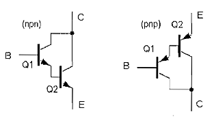
How to Identify Transistor Leads
First, set your multimeter to diode-test mode. Then test the leads two at a time. Where a connection exists between two leads (an internal diode), the multimeter will display a specific reading. The lead that connects to both of the other two leads is the base. If you identified the base using the positive (red) probe, the transistor is a positive type, or PNP; if you identified the base using the negative (black) probe, the transistor is a negative type, or NPN. Next, compare the readings the multimeter shows between base-collector and base-emitter - the lead showing the lower reading with the base is the collector, and the remaining lead is, naturally, the emitter.
How to Choose an Equivalent Transistor
To choose an equivalent or suitable replacement transistor, pay attention to its most important parameters:
- Maximum tolerable CE voltage
- Maximum current through CE
- Transistor power rating
- Transistor gain
- Transistor cutoff frequency
The points above should be considered in most cases. If you're choosing a horizontal-output transistor or a power-supply switching transistor, all of the above must be considered, along with the capacitance between B and C as well - since the higher the operating frequency, the more the capacitance between the transistor's leads matters. An important point when choosing power transistors is the current through E-C. In this case, the replacement transistor should not only tolerate this current, but should also be somewhat better than the original transistor, so it lasts longer in the circuit.
The table below lists the specifications of several transistors well suited for use as switches in circuits like these.
Relays
A relay is, in effect, a type of magnetically actuated switch that can use a small current to switch large electrical currents on and off. A relay is typically made up of a coil and metal contacts labeled N.C, N.O, and COM. The N.C contact is connected to the COM contact by default. When current flows through the coil, its iron core becomes magnetized and pulls in a metal armature - this action disconnects COM from N.C and connects it to N.O instead.
When working with relays, keep the following in mind:
When switching a relay on and off, the coil inside it (an inductor) generates a reverse voltage spike, which needs to be suppressed using a flyback diode. Take care that this diode isn't placed in a way that short-circuits the input. A relay has two rated voltages: one is the voltage applied to its coil, which can be 5, 6, 12, or 18 volts; the other is the voltage across N.C/N.O and COM, typically 220 volts. One of a relay's biggest advantages is its isolation - this keeps noise from the driven device and its actuators from leaking into the system's electronic circuitry. An important consideration is the relay's operating frequency: since a relay's switching action is mechanical, it has a severe frequency limitation, so a relay can't be switched thousands of times per second - which is why electronic components are typically used instead at high frequencies.
Power Supply Circuits
A robot's power supply is, in a sense, the robot's heart, since it's the source of energy for every other component. For mobile-base robots, we want to look at two types of power supply circuit.
Switching Power Supplies
First, let's review some definitions and look at a sample power supply.
1. EMI filter: This section consists of two components - an inductor, L1, and a capacitor, C1 - that together form a filter. This section serves two main functions:
Preventing radio-frequency emissions at the operating frequency, and keeping switching noise from being injected back onto the main supply line, Vin.
The other function is preventing spikes present on the Vin supply from entering the circuit. This filter's cutoff frequency shouldn't exceed 2 to 3 times the supply's operating frequency.
2. Input filter capacitor: This is a large capacitor responsible for storing energy, and it's made up of at least two capacitors: an electrolytic capacitor for the current components at the switching supply's frequency, and a multilayer capacitor for the harmonic and switching-frequency components.
Since wiring traces or PCB traces can be fairly long and exhibit significant impedance, having both of these capacitors is essential to keep the circuit stable while high-frequency current components pass through, and to supply the currents mentioned above. These capacitors need to be sized so that, at three times the supply frequency, they present negligible impedance.
3. Transformer: Besides providing DC isolation, this component also changes the voltage level. The voltage change is achieved by varying the turns ratio between the primary and secondary windings - but if the transformer design isn't right, it will affect circuit stability and the semiconductors' safety margins.
4. Power switch: This is usually a power transistor or MOSFET, operating in one of two states - fully on or fully off. Output voltage level is controlled by varying how long these stay on versus off. This, of course, is the most vulnerable part of the circuit - if any other part of the circuit misbehaves, this is usually the first part to get damaged.
5. Output rectifier: Responsible for rectifying the output voltage; in certain cases, discussed further below, fast-recovery diodes need to be used.
6. Output filter: Responsible for storing energy while the switch is on and delivering it to the load while the transistor is off - taking in energy during the on time and releasing it to the load during the off time. Roughly 50% more energy than the load actually needs gets stored in the inductor and capacitor.
7. Current-sensing sensor: The goal here is to produce a voltage proportional to the output current. This voltage is then amplified and used, through whatever method, to control the current.
8. Voltage feedback: a resistor-divider network taps a fraction of the output voltage and feeds it to the error amplifier for comparison against a reference voltage. Sensing the output voltage isn't limited to this approach alone, but it is a simple and common solution.
9. Control: this section's main job centers on generating PWM pulses and applying voltage and current feedback, along with soft-start (some important parameters in switching supplies are designed around the rated Vout, and when Vout is low, some components risk damage; passing through the transient stage and reaching steady state without damaging any part is called soft-start). It's made up of a waveform-generation section, a comparator working with ramp pulses, error amplifiers, and a voltage reference.
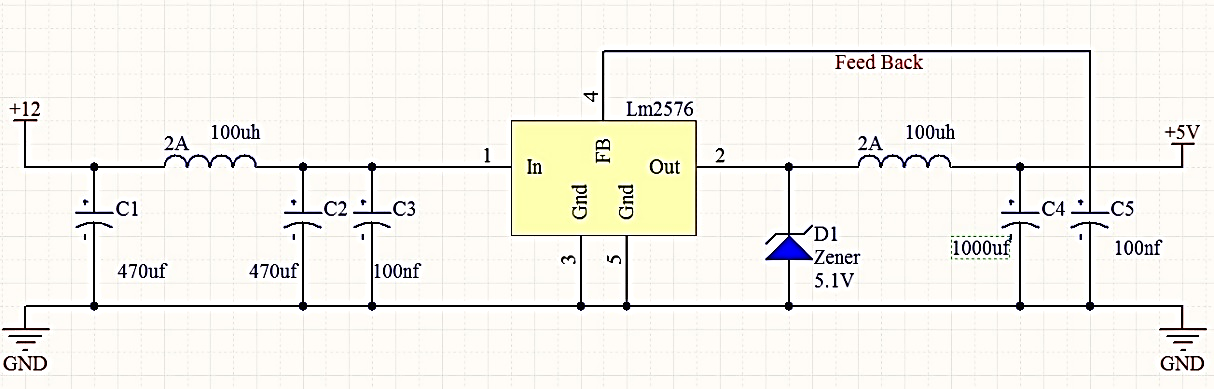
So that gives us an introduction to the principles, rules, and circuits of switching supplies. Fortunately, with the LM2576 IC - a switching power supply IC in its own right - power-supply headaches are considerably reduced. Below you can see this IC's schematic:
Because switching circuits convert the input voltage to the desired output voltage at high efficiency, unlike linear regulators such as the 7805, they don't run hot and don't stress the circuit.
Analog Power Supply
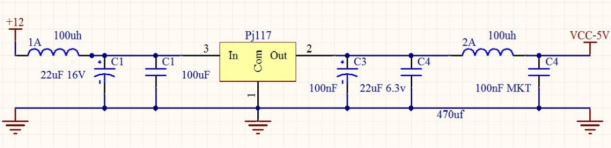
Figure 2-2: LM1117 - +5V
This circuit likewise uses an LC low-pass filter on both the input and output to filter current and voltage, and the results obtained from the sensors are excellent.
Distance Sensors
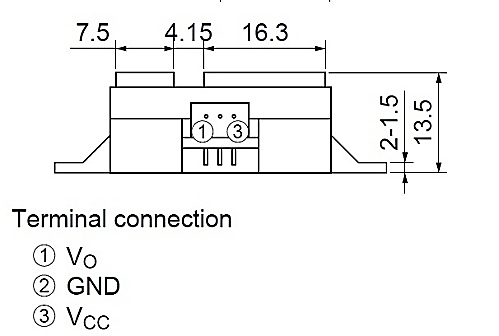
Over the years, Sharp has introduced a family of infrared sensors. These sensors benefit from small packages, very low consumption, and a variety of outputs. What follows is an overview of the different types within this sensor family, along with information on working with them and guidance on how to use them.
Theory of Operation
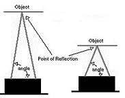
With the introduction of Sharp's GP2DXX sensor series, a new approach was introduced that not only extends the object-detection range compared with the previous method, but, in the case of the GP2D12 and GP2D120 sensors, also gives us range information directly. Thanks to their new distance-measurement methods, these rangefinders offer greater freedom from ambient lighting conditions. These new rangefinders all use triangulation together with a small linear CCD array to compute the distance to, or presence of, objects in the field of view. The basic idea is this: a pulse of IR light is emitted by the emitter. This light travels through the field of view and either strikes an object or continues on its path. If there's no obstacle (object), the light is never reflected back, and no range is reported. If the light reflects off an object, it returns to the sensor and forms a triangle between the reflection point, the emitter, and the sensor.
Figure 2-4: How the sensor works
The angles in this triangle change based on the distance to the object. The receiving section of these new sensors is essentially a precision lens, which directs the reflected light, according to the triangle's angle, onto different segments of the enclosed linear CCD array. The CCD array can determine the angle at which the reflected light returned, and can therefore compute the angle to the object. This new distance-measurement method is nearly immune to ambient-light interference, and shows a remarkable insensitivity to the color of the object being detected. Detecting a completely black wall in sunlight is now entirely possible.
Choosing a Sensor
The GP2XX sensors come in various derivatives. The table below helps identify each sensor type along with its maximum and minimum range, and whether the sensor in question delivers a variable distance reading or a boolean (true/false) detection signal. The GP2D15 and GP2Y0D02 (0D) models each provide a single digital value, in their own respective ways, based on object presence. None of these sensors require an external signal or timer - instead, they fire continuously, drawing a steady current of roughly 25 mA.
The A700 model is a special case, considerably larger than Sharp's other sensors. Its increased size accommodates larger lenses and circuitry needed for a maximum range of 5.5 meters. Which sensor to use depends on your application, on your controller's capacity (whether it has a spare A/D channel or not), and so on.
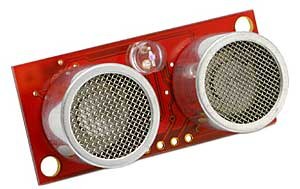
How Ultrasonic Sensors Work
An ultrasonic sensor uses ultrasonic waves to estimate distance.
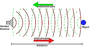
These sensors work by measuring the time interval between sending out a wave and receiving its echo, and, based on the speed of sound in that medium, estimating the distance to the obstacle. Ultrasonic sensors come in a range of types and see wide use across industry.
Figure 2-7
The frequency typically used in ultrasonic sensors is 40-60 kHz, which lies outside the range of human hearing. The main advantage of these sensors is that they detect objects using ultrasonic waves regardless of their color, shape, or surface finish.
H-Bridge Drivers
The most important consideration in controlling DC motors is controlling their direction. Using a single power supply (V+ and ground), H-bridge circuits drive a motor in both directions. Before looking at the components that make up these circuits and how to build them, let's look at how they work.
First, let's define clockwise (CW) and counterclockwise (CCW) direction by convention. Which direction is called clockwise and which counterclockwise is chosen arbitrarily.
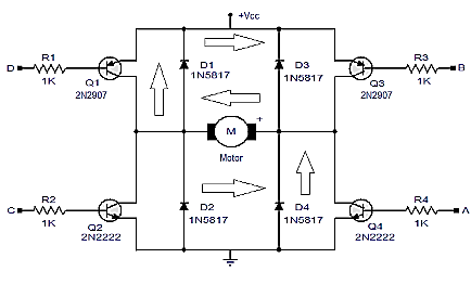
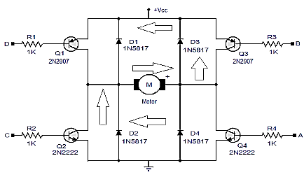
Figure 2-9 Figure 2-8
Figure 2-8 shows a common H-bridge circuit built with 4 transistors (this structure is presented purely to explain the concepts involved, so refrain from actually building it). To produce clockwise motion, transistors A and B need to be turned on. Figure 2-9 shows how current flows from negative to positive. The voltage applied to the motor is negative on the right side and positive on the left side. This circuit is named the "H" configuration because of how the transistors and motor are arranged. The H configuration also shows how input voltage is applied to the motor by turning transistors on and off diagonally. In Figure 2-9, turning on transistors B and C produces counterclockwise (CCW) current in the motor. Here too, the arrows indicate the direction current flows through the transistors and motor. Real H-bridge circuits operate on this same simple principle.
Back-EMF and Protection Diodes
DC motors are, by their nature, powerful inductors, and their inductive property causes plenty of problems in robotics projects. Inductors resist changes in current. When an inductor is connected to a power source and the voltage across it is suddenly cut off, it tries to keep the current flowing at its previous level. The faster the current is cut off (the faster the electromagnetic field's strength drops), the harder the inductor tries to resist. As a result of this effort, a potential difference (voltage) of up to 20 times (or more) the original voltage appears across the inductor's terminals (at the moment the main current is cut). The polarity of the voltage induced across the inductor (motor) is opposite that of the original voltage, and this is called back-EMF, or CEMF. CEMF arises the moment the magnetic field created by the original current suddenly collapses. We won't get into the physical intricacies behind this phenomenon here. Transistors typically can't withstand CEMF voltage spikes and burn out. Fortunately, circuits can be protected against CEMF. The most common protective method is using flyback diodes, installed in parallel with whatever's generating the CEMF. The flyback diode's job is to protect transistors from CEMF's negative effects. It does this by clamping the voltage down to about 0.6 volts, a safe level - and it's best if these diodes are a fast-recovery type.
Another Problem with Back-EMF
Using flyback diodes to protect transistors introduces another problem of its own. Current running in parallel with the main power path can generate transient voltage, or noise, on the PCB. What's more, if PWM (pulse-width modulation) is used to control the motors, CEMF current will occur on every on/off cycle. Sometimes, by the time the transistor turns back on, the CEMF current is still flowing. This happens where the transistor forms a direct path between ground and V+. The timing of this depends on how fast the flyback diodes are. This current is called "shoot-through current," and it's a source of noise. This is why it's especially important to place fast bypass capacitors (ceramic or tantalum) close to the H-bridge circuit - to protect the rest of the electronics and the battery. A bypass capacitor is an ordinary capacitor used to smooth out ripple (small fluctuations) and momentary transients on V+ (the power rail). Bypass capacitor values typically range from 0.1 to 0.22 microfarads.
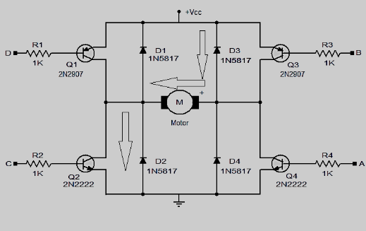
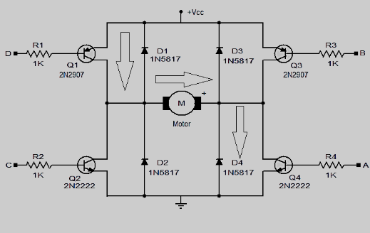
Figure 2-11 Figure 2-10
A capacitor is an electronic element that resists changes in voltage. A bypass capacitor is connected to the power-carrying conductor (which normally sits at VCC). When voltage fluctuations occur, the capacitor quickly absorbs energy, stabilizing the voltage. When the voltage sags, the capacitor discharges the energy it stored back into the circuit, raising the voltage back up. So when a bypass capacitor (typically 0.1 to 0.22 microfarads) is installed on an H-bridge circuit, the effects of this shoot-through current are significantly reduced.
A Simple (Low-Current) H-Bridge Circuit
Here's a simple H-bridge circuit for working with DC motors drawing 100 milliamps or less. This circuit's characteristics were covered in earlier sections. The resistor values are chosen conservatively, based on worst-case transistor gain. Once you're familiar with how this circuit works, you can design H-bridge circuits for higher currents. To do that, you'll need to swap in transistors and diodes rated for higher current, and you'll also need to adjust the resistor values for proper bypassing. Designing a new H-bridge circuit is a worthwhile exercise for robotics enthusiasts. This H-bridge circuit uses a 2N3904 NPN transistor on the high side and a 2N3906 PNP transistor on the low side. These transistors share matching characteristics in terms of gain, maximum current, and switching speed. Because of these similarities, they're used as complementary transistor pairs. The 1N5817 diodes tolerate high voltages and can carry up to 1 amp of current, which is usually well beyond what we actually need. 1/4-watt resistors with 5% tolerance work perfectly well in this application. The end result is a reliable H-bridge circuit. Despite its simplicity, this H-bridge circuit is quite capable and very easy to work with, since it has only two inputs (A and B). It also can't short-circuit - meaning both paths turning on and connecting V+ to ground - because the high-side and low-side transistors can never turn on at the same moment. Using PNP transistors on the high side also improves the circuit's efficiency. To operate this H-bridge, pull side A up to V+ and connect B to ground (Figure 2-21) - the motor then starts turning in one direction. To reverse the motor's direction, swap the A and B voltages. If you connect both A and B to V+ or to ground at the same time, nothing happens. Table 2-1 lays out all the states in practical terms - logic zero means ground, and logic one means the motor terminal is connected to V+.
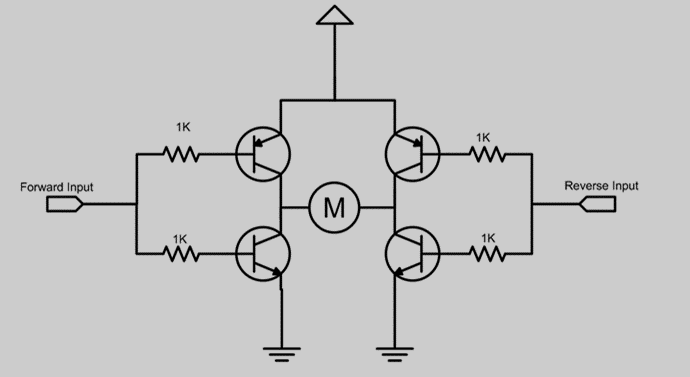
Table 2-1: H-bridge truth table Figure 2-12: Simple H-bridge circuit built with transistors
This is a versatile motor driver used to drive small motors. This IC can drive two DC motors or a single bipolar stepper motor (Figure 2-22). It supports voltages from 6 to 46 volts and can pass 2 amps continuously and 3 amps in transient peaks. It shuts itself off automatically on overcurrent and includes a current sensor. Everything you need to do is spelled out in the L298 datasheet. In this IC, the clamping diodes needed for proper operation sit outside the IC itself. In terms of its inputs, behavior, and physical appearance, the L298 closely resembles the L293 and the 754410. It's recommended to use 1N5822 diodes as the L298's clamping diodes.
L6203 Motor Driver
Like the L298, the L6203 IC uses an H-bridge circuit to drive DC motors. The main structural difference between the L298 and the L6203 is that the L6203 uses DMOS transistors instead of BJTs. DMOS devices, a special type of MOSFET, have a modified structure built for higher voltages and greater power handling. DMOS devices have a higher breakdown voltage (BVDS) than ordinary MOSFETs, but they carry the same drawbacks MOSFETs have. Generally speaking, BJTs have simpler operating regions and drive
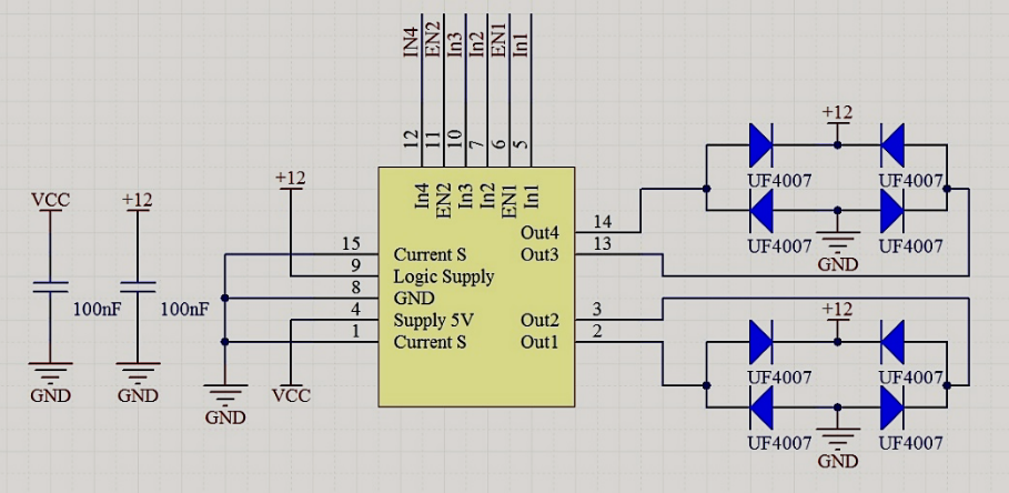
circuits face fewer constraints with them, but their current draw is higher, and their output current is capped at a specific limit - you can expect less power-handling capability from them than from MOSFET transistors when driving a DC motor, though this naturally depends on the specific BJT and MOSFET being used. On the other hand, MOSFET transistors need a minimum gate-source voltage of about ten volts to turn on (whereas with a BJT, we can turn the transistor on with a base-emitter voltage of around 1 volt) - but a MOSFET's input current draw is so low it can practically be treated as zero, so power dissipation is much lower, and we can deliver high output power.
Laser Scanners
A laser scanner lets you scan a wide area with high precision, identifying and localizing every obstacle present. One example worth mentioning is the URG-04LX laser scanner, a small, precise, reasonably priced scanner made by Japan's HOKUYO Corporation. This laser scanner is ideal for robotics applications. The URG-04LX model can scan distances from 20 millimeters to 4 meters across a 240-degree arc. This scanner's distance-measurement resolution is 1 millimeter, and its angular resolution is 0.36 degrees. This sensor's operating current, at 5 volts, is around 500 milliamps - a feature that makes it well suited for use in battery-powered systems.
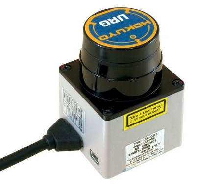
URG-04LX Laser Scanner Specifications
Operating range: 20 mm to 4000 mm
Short scan time: 100 milliseconds
Operating voltage: 5 volts
Scan angle: 240 degrees, with 0.36-degree angular resolution.
USB and serial (RS232) interface support for maximum flexibility
Thermal Array Sensor
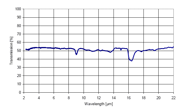
The TPA81 is a precise temperature sensor suited for industrial, robotics, and similar projects. This sensor is an infrared-detecting thermopile array covering the 2-22 μm range, and it provides a matrix of the temperatures in front of it; this sensor can also detect temperatures from 12 to 100 degrees Celsius depending on distance. Its communication protocol is I2C.
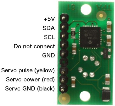
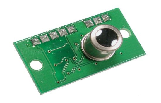
Figure 2-14: TPA81 sensor
Thermal Imaging Sensor
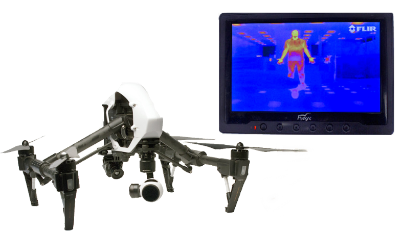
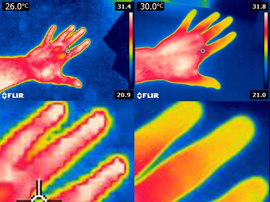
A thermal (infrared) imager is a device that produces images by measuring infrared radiation, whereas an ordinary camera produces images by measuring visible light. It also goes by other names: thermal infrared camera, thermal imaging camera, heat-measuring camera, or infrared-radiation-sensing camera. Visible light's wavelength runs from about 400 to 700 nanometers, so an ordinary camera measures light intensity in roughly that wavelength range; a thermal imager, however, measures the intensity of electromagnetic radiation at wavelengths around 14,000 nanometers and beyond. Infrared energy is just one part of the electromagnetic spectrum, which also includes gamma rays, X-rays, ultraviolet, the thin band of visible light, infrared, terahertz waves, and short and radio waves. There are many similarities and differences among these wavelength bands, and all of them emit a characteristic amount of blackbody radiation as a function of temperature. Generally speaking, a thermal camera can find its way around much like an ordinary camera that uses visible light, and it even works in complete darkness, since the amount of available light doesn't matter to it at all - which makes it useful for firefighting operations inside smoke-filled buildings and in underground passages. Images from thermal cameras tend toward monochrome, because these cameras are typically built with just one type of sensor responsive to a single infrared wavelength band. Color thermal cameras require a more complex design with multiple different wavelength bands and carry less meaning outside the normal visible spectrum, since different wavelengths aren't rendered the way the human color-vision system perceives them. These monochrome images are sometimes displayed in false color, where color changes are used more to represent changes in contrast than changes in the underlying signal - useful because humans have a much wider range for perceiving contrast than for perceiving color across its full range. Better contrast perception in bright regions is a reasonable limitation of this technique, called contrast enhancement. For temperature measurement, the brightest part of the image, normally shown in white, shifts to somewhere between red and yellow, while the coolest part is rendered dark blue. A given standard should show the image in false color tied consistently to temperature-dependent colors. Their resolution is markedly lower than that of optical cameras - often just 160×120 or 320×240 pixels - and thermographic cameras are far more expensive than their visible-spectrum counterparts. High-end models are typically treated as dual-use and subject to export restrictions. In uncooled detectors, the temperature differences between the sensor's pixels are small - around 1°C - while the inferred temperature resolution is only about 0.03°C different from the sensor itself. Pixel response time is gradual, on the order of 10 milliseconds. Thermal imaging has plenty of other applications too. For example, firefighters use it to see through smoke, locate people, and localize hotspots within fires. Thermal imaging is also used in power-line maintenance to identify sections and joints that are running abnormally hot, revealing telltale signs of a developing fault before it becomes a serious hazard. In buildings where thermal insulation has failed, this technique can reveal where heat is leaking through, helping improve the building's response to hot or cold weather conditions. Thermal cameras are installed in a number of luxury vehicles to assist the driver. Certain physiological processes and specific responses in humans and other warm-blooded animals can also be studied using thermal imaging. Infrared cameras are also found on most research telescopes used in astronomy.
Passive Infrared Sensors
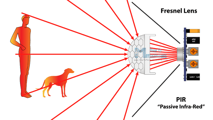
"Passive infrared sensors" are electronic devices that measure infrared radiation from objects and targets within their field of view. These sensors are called "PIR sensors," short for Passive Infrared sensors.
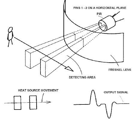
PIR sensors are sometimes used to detect moving targets: an infrared source at one temperature, such as a body, passes in front of another infrared source at a different temperature, such as a wall, and detection is based on this change. Every object emits infrared radiation. This radiation is invisible to humans, but it can be detected using electronic devices built for that purpose. The word "passive" in this sensor's name means the sensor itself emits no energy of its own - it only receives infrared radiation through its sensor face. At the core of a PIR sensor sits one or a small group of semiconductor sensing elements, with a surface area of roughly a quarter of a square inch. This region is made from pyroelectric material.
Kinect
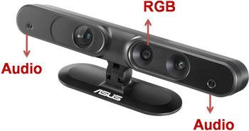
Kinect for Xbox 360 - or simply Kinect, originally known during development as Project Natal - is a device that enables playing video games without using any kind of controller at all. Its use isn't limited to video games, either; it can be used for all kinds of entertainment, such as watching movies and listening to music. The device was built by the American company Microsoft and works with the Xbox 360 game console.
The device is built around a camera with two lenses along with an infrared port: the infrared port and one of the cameras handle depth detection, while the other camera, an RGB color camera, handles image recognition. This camera lets Xbox 360 users control everything on screen without touching any controller at all. It can even understand and recognize the user's voice, and carry out commands issued by the user based on that recognition. The device went on sale in North America starting November 4, 2010.
7 Uses for Kinect
In 2011, Microsoft's Xbox 360 game console sparked a huge revolution in the gaming industry with its motion sensor, Kinect. Kinect is a device capable of recognizing motion and voice, built around a set of infrared cameras and microphones that filter out extraneous ambient noise. This motion sensor sees users and interprets and simulates, say, a hand motion as a tennis racket swing, or a leg motion as a kick toward a goal. In this way, the technology figures out where the user is standing, then reads their body position and movements and, with the help of a computer, converts them into control commands. Microsoft achieved enormous success with Kinect's launch - from Kinect earning a spot in the Guinness World Records for its extremely high sales, to opening up a whole new outlook on gaming and device control. Today, Kinect's applications, well ahead of their time when it launched, have gone far beyond controlling Xbox 360 games, and this technology has found some fascinating and unexpected uses. Hundreds of ideas have been built around Kinect technology - we'll mention just a few examples here:
1. Personal Computers
Given how important touch-and-motion tools have become, Microsoft, the maker of the Xbox console, intends to release Kinect for Windows too. The Windows version of Kinect will likely differ from the Xbox version, and it will be supported by Windows 8 and Microsoft development tools such as .NET 4.5 and Visual Studio. Xbox Kinect can detect movement from several meters away, whereas the PC version of Kinect will be limited to around 50 centimeters. Imagine that, before long, you'll be able to mount a Kinect sensor above your monitor at home or at work, and no longer need a mouse to navigate software environments.
2. Operating Rooms
Recently, at Sunnybrook Hospital in Canada, Xbox Kinect has found its way into the operating room - not for playing games during surgery or relieving doctors' fatigue, but to assist them during surgical procedures. Surgeons sometimes need to review a patient's CT scan or MRI images again mid-operation. Doing so traditionally meant stepping into an adjacent room to view the images on a computer, then, before returning to the operating room, scrubbing in again and repeating every step required for sterility. This process adds roughly 20 minutes to an hour to the procedure's total time. But thanks to an innovation implemented at this hospital, surgeons can now use Kinect to view images on surrounding displays and flip between images using motion commands, all without ever leaving the operating room. This keeps surgeons focused and saves both time and cost. Interestingly, researchers at Mashhad University of Medical Sciences have likewise designed a system for accessing patient information during surgery using Kinect technology.
3. Modeling
Not long ago, MIT released a video showcasing one of Kinect's most fascinating applications. In this project, called inFORM, when a person moves their hands, the Kinect camera sends that data to a dynamic surface, and an array of square pegs embedded in it moves up and down in response. The video shows these moving pegs able to bounce a ball, but this technology can produce plenty of other kinds of motion too. MIT researchers believe this technology could have practical applications in geospatial data - including maps, GIS (Geographic Information Systems), terrain models, and engineering models.
4. Virtual Conferencing
Sit at home and send your avatar to meetings instead. An avatar is an image internet users, particularly on forums, use to represent themselves. Kinect recognizes your movements and behavior and transfers them onto your avatar, letting you hold your meeting from home or anywhere else.
Another use for Kinect's video-conferencing technology is video consultations with patients who can't make it to medical clinics in person. In this project, instead of seeing actual video footage of patients, doctors see cartoon avatars of them, resembling Xbox Live avatars. Even so, doctors can still diagnose their condition and prescribe the necessary treatments and medications remotely.
5. Aerospace
You've surely heard of Curiosity, NASA's most recent Mars rover. The Mars landing operation was nicknamed "seven minutes of terror," and landing a robot on a planet 53 million kilometers from Earth truly is terrifying. Even the smallest glitch during landing could have burned Curiosity up or shattered it on impact with the Martian surface, wiping out months of effort and planning. So NASA turned to Microsoft's Kinect for help. A simulation of Curiosity's eight-minute descent was built, controlled entirely through Kinect. NASA ran this project repeatedly to work out the best possible response for bringing Curiosity's eight-month journey to a safe conclusion. This joint NASA-Microsoft project was called Mars Rover Landing, and it's now available to Xbox users as a game.
6. Automobiles
Who knows - before long we might be driving cars that respond to the driver's body, hand, and facial movements. Evidence suggests Microsoft is preparing this technology for major automakers such as Ford, Fiat, and Kia. The motion sensors in these vehicles will be smart enough to recognize the driver and, using advanced data-analysis techniques, offer new approaches to vehicle guidance and assessing its current condition. To that end, Microsoft unveiled a concept car the previous year at America's annual Detroit auto show. This car uses Kinect technology, Xbox 360, Windows Phone, the Bing search engine, and more. Among this vehicle's features are Kinect cameras built into the taillights, giving the driver a live view of the area around the car. Cars will likely become so advanced in the future that the driver's attention will no longer even be on driving itself.
7. Robotics
A fundamental trait of robots is the ability to interact with their surroundings, usually by perceiving the environment with the help of sensors. The Kinect sensor provides robots with 3D vision as well, which is why scientists have used Kinect as a robot's "eye." With a Kinect sensor and the help of image- and audio-processing software, a robot can be equipped with sight and hearing. Numerous robots have been built using Kinect technology to date. For example, in a research project in Zurich, a flying robot is controlled by body movements with Kinect's help. Another company has built a household robot called SmartPal VII that uses Kinect technology to mimic the limb movements of its users. This robot is designed for the elderly and people with disabilities, helping them handle daily tasks and move objects around with ease.
Inertial Measurement Unit (IMU)
Controlling and navigating a mobile robot isn't possible without knowing its position. Various sensors have been designed and built for this purpose, each suited to a particular application. Types of positioning systems include the precision accelerometers used in missiles, the gyroscopes found in aircraft, altimeters, direction-finding systems based on Earth's magnetic field, GPS-based positioning systems, positioning systems using electromagnetic or acoustic wireless networks, and even highly sophisticated star-tracking positioning systems used aboard satellites and spacecraft.
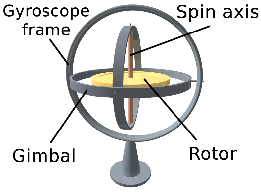
The rise of MEMS technology has had a dramatic effect on shrinking the size and cost of various electromechanical sensors while improving their accuracy. This makes it possible to fit multiple sensors into a single small robot. In some cases, manufacturers even package several positioning sensors (such as an accelerometer and a gyroscope) into a single chip. Among positioning devices, sensors that measure acceleration, angular velocity (gyroscopes), and magnetic field are the most widely used components in small autonomous robots. This section of the book focuses on the accelerometer module and the gyroscope module. Using an accelerometer, you can compute a robot's acceleration, and, by integrating, its velocity and position as well. Keep in mind that Earth's gravitational acceleration (g) also factors into an accelerometer's readings. This complicates positioning, but it's useful for measuring deviation from the direction of gravity (the vertical). A gyroscope, meanwhile, fundamentally measures angular velocity, and by integrating that, you can also compute angular position (orientation). Combining an accelerometer and a gyroscope this way lets you measure your mobile robot's position and orientation, and, in particular, how far it has tilted from vertical (the direction of gravity).
Accelerometer
Every MEMS accelerometer, in one form or another, contains an internal proof mass that moves under the influence of external force. This mass is held in place by a spring-like structure, and its displacement under external force is measured through various methods, such as changes in capacitance. Once you know the spring structure's stiffness constant and the proof mass's value, this displacement is converted into an equivalent acceleration. Given this, MEMS accelerometers inherently measure the external force applied to the proof mass. Because of this, every accelerometer of this type measures static acceleration (Earth's gravity) and dynamic acceleration (from changes in velocity) in exactly the same way, and separating these two measured values is left up to you. So if your accelerometer's measurement axis is aligned with gravity, the measured value reflects acceleration from motion plus gravitational acceleration (9.8 m/s²); but if the sensor's measurement axis is horizontal (perpendicular to gravity), only dynamic acceleration is measured, and gravity has no effect on the reading. So if a system uses a single-axis accelerometer (capable of measuring along only one coordinate direction), you need to know its mounting angle relative to gravity's direction in order to account for the static-acceleration contribution.
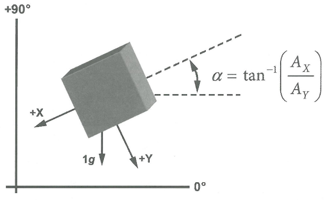
Now imagine you have two or three accelerometers whose measurement axes are pairwise perpendicular to each other (like the X, Y, and Z axes in a standard Cartesian system). If this assembly's velocity is constant and only the static acceleration from gravity acts on it, comparing the ratio of the acceleration measured along each axis lets you compute this assembly's mounting angle relative to gravity's direction. This is the method used in many electronic levels and mobile robots to measure orientation angle relative to gravity's direction.
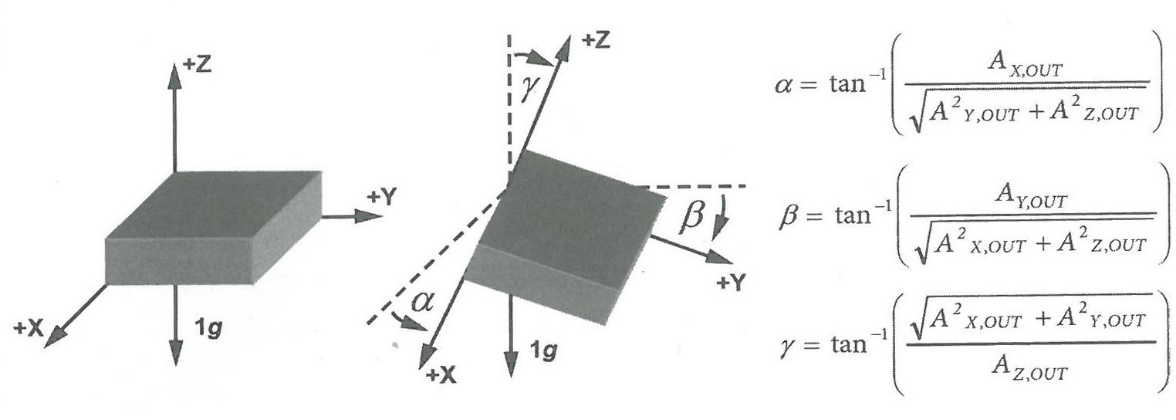
Figure 2-23: Using a three-axis accelerometer to measure the direction of Earth's gravity in three-dimensional space. In this figure, the three-axis accelerometer's (X-Y-Z) orientation relative to the horizontal plane and gravity's direction can be computed using the given equations. Note that knowing the angles between each axis and gravity's direction doesn't by itself give the accelerometer's complete angular position in three-dimensional space. In fact, if this accelerometer is rotated about an axis parallel to gravity, all three of its axes will measure the same results as before. To fully determine the accelerometer's angular position, at least two known, non-parallel vectors (the gravity vector and one other vector) need to be measured by it. In any case, a three-axis accelerometer can be used to build an electronic level capable of measuring tilt along two perpendicular directions. Many manufacturers produce two-axis and three-axis accelerometers as a single chip, made up of two or three accelerometers, respectively, mounted along mutually perpendicular directions in one package.
One of the fundamental drawbacks of using an accelerometer to measure tilt is that dynamic acceleration (from changes in velocity) affects the orientation reading. For example, if you mount such a device in a car to measure road grade, the measured direction is correct as long as the car's speed stays constant - but the moment the car's speed changes, the dynamic-acceleration vector adds to the static-acceleration vector, and your measuring device ends up measuring the direction of this new combined vector (which differs from gravity's actual direction). Other drawbacks of accelerometers include high sensitivity to vibration and noisy output.
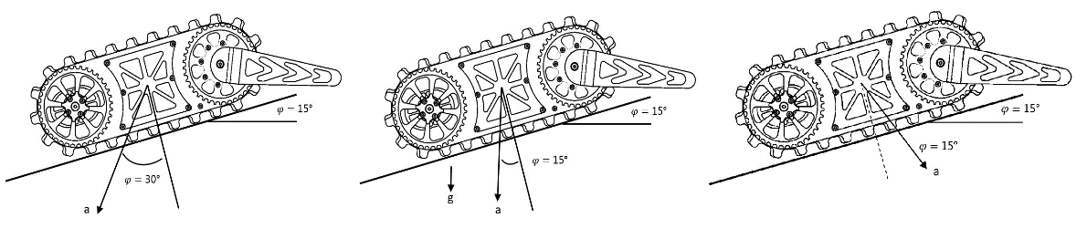
Figure 2-23: Measuring road grade by having a car-mounted accelerometer measure gravity's direction. The car's motion in figure (a) has positive acceleration (speeding up), in figure (b) has no acceleration (constant speed), and in figure (c) has negative acceleration (braking). As you can see, only in figure (b) is gravity's direction - and therefore the road's grade - measured correctly.
This sensitivity to vibration and dependence on dynamic acceleration makes it necessary to draw on other sensors as well, such as a gyroscope and a magnetic-field sensor (electronic compass), to measure gravity's direction reliably.
When choosing an accelerometer, pay attention to the measurement range you need, the sampling rate, how it communicates (analog or digital, and which communication protocol), and how many axes your project requires (one-, two-, or three-dimensional). Other parameters worth considering in MEMS accelerometers include sensitivity to temperature changes and supply-voltage variation, and initial offset (the reading at zero acceleration), which needs to be corrected through calibration. The following sections introduce how to use a three-axis (3D) accelerometer.
Gyroscope
As you know, a gyroscope fundamentally measures angular velocity about an axis: rotation about an axis is measured as a specific value (usually in degrees per second, deg/s), rotation in the opposite direction produces a result with the opposite sign, and when rotation stops, the measured value is zero. (Mechanical gyroscopes, which work based on the Coriolis forces of a spinning mass, were used in aircraft and missiles for a long time, until optical gyroscopes and various MEMS types were developed. Among the types developed, optical gyroscopes are the most precise, and MEMS gyroscopes are the cheapest and most widely used type of this measuring device.) Unlike an accelerometer, a gyroscope generally isn't sensitive to vibration and produces more consistent measurement results. But since angular velocity alone isn't very useful on its own, and most mobile machines care more about angular position, this sensor's output is integrated to derive angular position. Because gyroscope-based positioning systems rely on an integrator, even the smallest offsets and persistent errors - which are unavoidable - accumulate over time and produce substantial error. As a result, the angular position computed by integrating the gyroscope's output drifts further and further from its true value over time, to the point that after a few minutes (or even a few seconds), the computed value becomes completely invalid.
This makes it necessary to use gyroscopes alongside other sensors, such as Earth's-magnetic-field direction sensors or an accelerometer - unless the goal is purely to measure rotational speed rather than angular position, in which case the integrator can be dropped and the gyroscope's output will be accurate enough on its own. Like MEMS accelerometers, MEMS gyroscopes are built at very small sizes and reasonable cost, and many manufacturers even package two or three gyroscopes, mounted along mutually perpendicular directions to measure along different axes, into a single electronic chip.
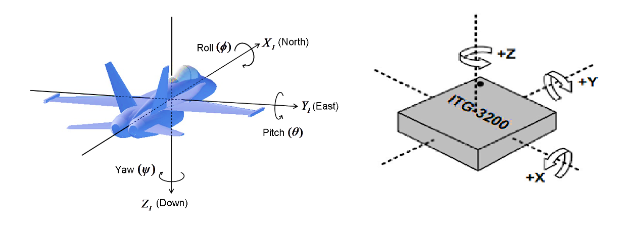
Figure 2-24: A three-axis gyroscope measures rotational speed about three mutually perpendicular axes. Clockwise rotation about each axis is usually denoted with a positive sign, and counterclockwise rotation with a negative sign. Rotational speed is often expressed in degrees per second (deg/s). In aircraft such as missiles and airplanes, as well as in some mobile robots, the terms Roll, Yaw, and Pitch are used to denote the rotation axes. The Roll, Yaw, and Pitch axes don't necessarily align with the coordinate axes - this depends on how the coordinate axes are assigned to the moving body.
When choosing a gyroscope, pay attention to its measurable speed range, sampling rate, how it communicates (analog or digital), and how many axes your project's application requires (one-, two-, or three-dimensional). Besides the parameters just mentioned, things like sensitivity to temperature changes and supply-voltage variation, initial offset (the reading at rest), and sensitivity to rotation along directions other than the measurement axis are all points that deserve attention.
Fusing Accelerometer and Gyroscope Output Data
In this section, we want to use gyroscope and accelerometer data together to correctly determine gravity's direction. A two- or three-axis accelerometer can be used on its own to measure orientation relative to gravity's direction (Figures 1 and 2), but this measurement is only accurate if no acceleration other than gravity's static acceleration acts on the system. That's not achievable in mobile robots. On top of that, an accelerometer is highly sensitive to vibration, and because of its heavy noise, its output data isn't worth much on its own. The gyroscope, for its part, has its own drawbacks - most notably that the angle computed through integration gradually drifts away from the true value. Fortunately, the errors present in gyroscope and accelerometer measurements have entirely different characters, so that by properly combining both sensors, the output errors of each can be corrected. To make effective use of data from both sensors, you need to fuse their output in a way that produces a result more reliable than either sensor's data on its own.
Various algorithms have been developed for fusing sensor data. Among them, the Kalman algorithm is one of the best approaches, usually known as the Kalman filter. The Kalman filter works by taking in noisy measurement data from a set of sensors and, knowing each sensor's uncertainty (noise variance), estimating the true value of the measured parameter with better accuracy (lower variance) than any single measurement. This filter is recursive in nature, and to produce its output it needs both the current measurement and data from the previous step. After estimating the measured variable, the Kalman filter produces its output based on a weighted average of the sensor measurement and the estimated result, and in this process, whichever source has greater certainty (lower variance) has more influence on the output. The Kalman filter's weighting coefficients aren't fixed - they're recomputed at every step for use in the next one. Using the Kalman algorithm requires knowing each sensor's (gyroscope and accelerometer) uncertainty, as well as heavy matrix-based mathematical computation that's beyond the capability of many microcontrollers. For this reason, small projects generally use a simplified version of the Kalman filter or other, simpler data-fusion algorithms. Below, we describe two methods that can be implemented on a microcontroller. To remove the noise present in accelerometer measurements, you could use a low-pass filter (or an averaging filter), but this filter introduces a lag in the measurement, and any lag in a control system reduces the overall system's stability. What's more, with this approach, acceleration caused by actual motion (as opposed to vibration) isn't removed by the filter, and this leads to an incorrect calculation of gravity's direction.
Control Principles
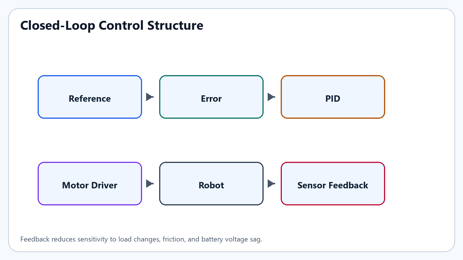
In robotics, we deal with mechanical structures as the systems we want to control. Mechanical systems, though enormously varied, share roughly similar principles when it comes to controlling them. To understand and control complex systems, we need to work out the relationship between the system's inputs and outputs, and derive its mathematical model. Systems are often dynamic in nature, and the equations describing them are usually differential equations. In controlled systems, unwanted, intrusive inputs that push the system away from the desired condition are called disturbances. Disturbances may enter through the input, alongside the reference signal, or through other parts of the system. In control theory, the goal is to implement specific measures so that, despite whatever disturbances exist, the system's behavior tracks only the reference signal. Various control systems have been designed for this purpose.
Types of Control Systems
Control systems fall into two categories: open-loop (without feedback) and closed-loop (with feedback) (Figure 4-1). In an open-loop system, the reference signal is applied to the system's input, and the controller generates an output signal based on it. Ultimately, the controller's output signal drives the actuator, and this element acts on the system. But there's no guarantee the system will behave the way we want - a disturbance or intrusive input can affect the system's behavior. Consider, for example, an electric motor whose shaft has seized in place because of a mechanical fault. In this case, the controller applies a motion signal to the actuator (the motor) based on the reference input, but the motor's shaft still doesn't move. So open-loop control systems are used where the system's behavior is fully known and the environment is free of any disturbance. A closed-loop system, by contrast, has a measuring element that samples the system's current state (its output) and feeds the result back as a feedback signal to a summing junction. The summing junction then generates an error signal based on the difference between the reference signal (the desired condition) and the feedback signal (the actual condition), and this error signal drives the controller and the stages that follow. The constant goal is to reduce this error signal and bring the actual condition closer to the desired one.
In control theory, four characteristics of a closed-loop system's response to a step input matter a great deal.
They are:
- Rise time: the time needed for the system's output to reach 90% of its final (desired) value.
- Overshoot: the difference between the response's peak value (maximum amplitude) and the desired value
- Settling time: the time needed for the system's response to converge to its final value.
- Steady-state error: the difference between the system response's final value and the desired value in steady state.
The constant goal is to improve the system's transient and steady-state characteristics - meaning we aim to reduce rise time, settling time, overshoot, and steady-state error as much as possible. Of course, changing any one of these parameters affects the others, so we need to strike a balance between these characteristics and the cost of building a better controller.
Various controllers have been built based on different techniques for correcting error and improving the transient and steady-state response. We'll look at a few types of these next.
Two-Position (On/Off) Controllers
This controller's output signal can only sit in one of two states: off or on - if the error signal is positive (the current condition is below the desired condition), the controller's output turns on and drives the next stage (the actuator). A common example of this controller is the thermostat in heating systems. A two-position controller with these characteristics has one major flaw: with the slight oscillation around the desired condition that's unavoidable because of environmental disturbance, the error signal keeps flipping sign, and the controller's output keeps switching on and off. In some situations, this can wear out the controller and the actuator. To overcome this problem, two-position controllers are built with a dead band: each time the error signal flips sign, if its magnitude doesn't reach a certain threshold (the dead band), the controller's output doesn't change state. So at the cost of a slight increase in error, the controller's and actuator's needless oscillation is significantly reduced.
Two-position controllers are simple and cheap, but they have low precision, and even with a dead band, some amount of error always remains in the system. Even so, in processes that don't need much precision, a two-position controller is a solid choice. Figure 4-3 shows the signals for a typical closed-loop system using a two-position controller.
Proportional (P) Controllers
If the output signal reflects not just the error signal's sign but its magnitude as well, we get a proportional controller, whose action scales with the error signal, and which can therefore correct error far better than a two-position controller. This is a proportional controller's core idea. The relationship between a proportional controller's input and output signal is as follows:
where e(t) is the error signal, u(t) is the controller's output signal, and kp is the proportional gain. One drawback of proportional controllers is that the system will still have some steady-state error once it settles, since a proportional controller can't eliminate error completely. Of course, increasing the proportional gain Kp reduces the steady-state error - but it also increases the system's oscillation and the risk of instability (Figure 4-4).
Eliminating steady-state error in a closed-loop system using a proportional controller was the idea behind building integral controllers.
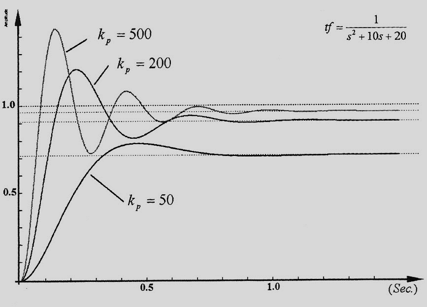
Figure 4-4: A typical closed-loop system's response to a step input with a proportional controller. Increasing kp reduces rise time and steady-state error, but increases overshoot and the risk of instability.
Integral (I) Controllers
In an integral controller, the controller's output signal at any moment is proportional to the integral of the error up to that moment. This integrating property eliminates steady-state error, and the system's output eventually matches the desired value. One drawback of this controller is its slow response, which is why it's generally not used on its own but alongside a proportional controller, as a proportional-integral controller. The mathematical relationship between a proportional-integral controller's input and output signal is as follows:
where u(t) is the controller's output signal, e(t) is the error signal, kP is the proportional gain, and ki is the integral gain.
Using a proportional-integral controller eliminates steady-state error and reduces rise time, but it increases settling time and overshoot (Figure 4-5).
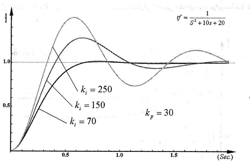
Figure 4-5: A typical closed-loop system's response to a step input with a proportional-integral controller. Increasing the integral gain ki reduces rise time, but increases settling time and the risk of instability.
Generally, when using a proportional-integral controller, we choose a smaller proportional gain Kp than we would if using a proportional controller alone, since the integral controller also reduces rise time and increases overshoot (much like the proportional controller).
Derivative (D) Controllers
This controller's output signal responds to changes in the error, and since a change in error can be an early sign of growing error, a derivative controller alone can't reduce it - so this controller isn't used on its own, but generally alongside a proportional controller, as a proportional-derivative controller. The mathematical relationship between a proportional-derivative controller's input and output signal is as follows:
where u(t) is the controller's output signal, e(t) is the error signal, kP is the proportional gain, and kd is the derivative gain. A typical closed-loop system's response with a proportional-derivative controller is shown in Figure 4-6.
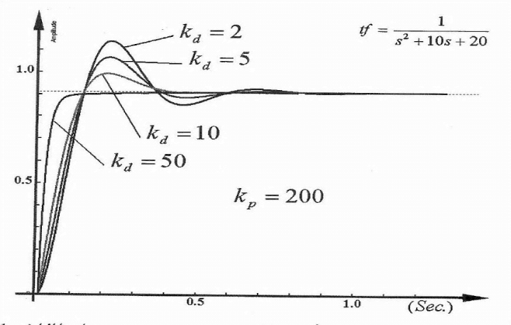
Figure 4-6: A typical closed-loop system's response to a step input with a proportional-derivative controller. As we can see, the derivative controller reduces overshoot and settling time, and has a small effect on rise time too, but it has no effect on steady-state error. Increasing the derivative gain Kd too much increases settling time again, so it's undesirable.
The PID Controller
The PID controller has, to date, been the most common error-correction algorithm in control systems - more than 90% of control loops worldwide are currently of the PID type. As technology has advanced, PID controllers have come a remarkably long way - from mechanical, pneumatic, and electropneumatic controllers, to electronic controllers built with vacuum tubes and transistors, and today, in the form of microprocessor-based systems and integrated circuits. The rise of microprocessors had a dramatic effect on PID controllers, to the point that most PID controllers built today have a microprocessor-based architecture.
As the name suggests, a PID controller combines three components: P, I, and D. The mathematical relationship between this controller's input and output signal is as follows:
where u(t) is the control signal and e(t) is the control loop's error. The controller's signal has three components: a proportional term (proportional to the error), an integral term (proportional to the integral of the error), and a derivative term (proportional to the derivative of the error). The controller's parameters are the proportional gain KP, the integral gain Ki, and the derivative gain Kd. The proportional term acts on the system's current error, the integral term accounts for the average of past errors, and the derivative term predicts future errors through linear extrapolation (Figure 4-7).
But designing a good PID controller goes far beyond what's been described so far. Simply implementing the PID mathematical relationship doesn't necessarily produce a good controller. To design a good PID controller, the following points need to be considered:
- Noise's effect on the derivative controller
- The effect of the reference signal
- Integral windup
- Tuning the controller's gains
- Computer implementation
Noise's Effect on the Derivative Controller
Differentiation is always sensitive to noise, and it amplifies high-frequency noise present in the error signal far more than the error itself. This means noise present in the system (usually generated by the feedback sensor) can create heavy oscillation in the control signal. So the measured signal (or the error signal) needs to be passed through a low-pass filter to remove its high-frequency noise.
The Effect of Reference Signal Changes
Any change the user makes to the reference signal causes a sudden change in the error signal, and because the derivative controller is sensitive to sudden changes, this can cause a very large, needless sudden change in the control signal - which ultimately saturates the controller and the actuator. So the reference signal is also passed through a low-pass filter before entering the loop, so that sudden changes in the reference signal don't cause needless oscillation in the controlled process.
Integral Windup
Even though many aspects of a control system can be understood using linear theory, certain nonlinear phenomena need to be accounted for in a practical controller. Windup is one such phenomenon, arising from the interaction between integration and saturation. Every actuator has limits - an electric motor, for example, has a speed limit. In a control system covering a wide range of operating conditions, situations can sometimes arise where the control signal drives the actuator right up against its limits. When this happens, the feedback loop effectively breaks, and the system behaves like an open-loop system, since the actuator's action stays pinned at its saturation limit regardless of the process's actual current output and error signal. In this state, if an integral controller is in use, the control signal keeps growing larger and larger - the controller, so to speak, winds up. It then takes a long stretch of opposite-signed error before the controller returns to its normal (closed-loop) behavior. So once the actuator saturates, controllers that include an integrator can cause an extended transient and a large settling time.
Figures 4-8 and 4-9 illustrate the windup phenomenon in a typical process controlled by a PI controller. In the chart in Figure 4-8, a change in the reference signal at time zero (a step from zero degrees) drives the actuator into heavy saturation. The integral term keeps growing, since the error is positive, and it reaches its maximum right at the moment the error hits zero. At this point, because the integral term is so large, the actuator stays saturated. The actuator doesn't come out of saturation until the error has been negative long enough to bring the integral term down to a reasonable level. As we can see, the control signal swings back and forth several times between its positive and negative limits. The system's response shows a large overshoot that damps out after several oscillations. Eventually, the system's output settles around the desired value, and the actuator recovers from saturation back into its normal closed-loop operation.
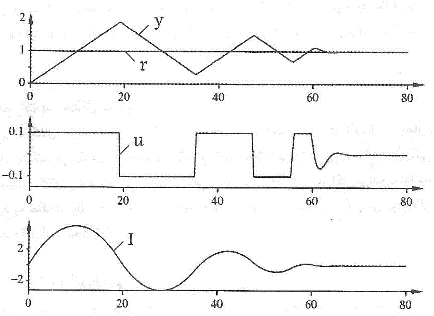
Figure 4-8: Because the integral term winds up, the controller's output oscillates needlessly between its positive and negative saturation states, and the system's output ends up somewhat oscillatory as a result.
Choosing the reference signal poorly can saturate the controller and cause windup. In the chart in Figure 4-9, the reference value sits beyond the actuator's saturation limit right from the start, so the system's output can never reach the desired value. With the actuator saturated, the integral term keeps growing continuously (winding up). Now, if the reference signal drops down to a smaller value, below the actuator's saturation limit, the actuator still stays saturated until the error signal has been negative long enough for the integral term to shrink back down. The more an integral controller has wound up, the longer it takes to return to normal. In this case, on top of the control loop breaking due to saturation, settling time also increases, which is undesirable. Figures 4-8 and 4-9 illustrate the controller-windup phenomenon resulting from reference-signal changes and from choosing a reference signal beyond what's achievable. This phenomenon can also arise from large disturbances or equipment faults. There are various ways to counter windup, including placing limits on the reference signal so the actuator never reaches its saturation limit, and halting integration whenever the actuator is saturated.
Tuning the Controller's Gains
When implementing a PID controller, the gains kP, ki, and kd need to be tuned correctly so the system's behavior matches what we want. To do this, it's enough to obtain the process's open-loop response to a step input, then, by adding proportional, derivative, and integral control to the closed-loop system, improve rise time, overshoot, and steady-state error, respectively. As a general rule, consider the table below.
| Closed-Loop Response | Rise Time | Overshoot | Settling Time | Steady-State Error |
|---|---|---|---|---|
| Proportional gain kP | Decrease | Increase | Small effect | Decrease |
| Integral gain ki | Decrease | Increase | Increase | Eliminate |
| Derivative gain kd | Small effect | Decrease | Decrease | Small effect |
Various methods exist for estimating an initial value for the controller's gains. The best known are the step-response and frequency-response methods, put forward in 1940 by Ziegler and Nichols. Describing these methods is beyond this book's scope.
Computer Implementation
Today, most controllers are implemented digitally, in computers and microcomputers. In this section, we'll describe how to implement a PID controller on a digital computer (microcontroller). When a controller is implemented on a digital computer, sensor readings are sampled at specific times, and the resulting output appears at the computer's output, and gets applied to the actuator, after a certain delay. Compared with an analog implementation, this is a drawback, since sampling at fixed time intervals introduces dead time into the control loop and produces sampling error. To reduce sampling-related error, the sampling frequency needs to be much higher than the frequency of the controlled process's dynamic parameters (in theory, at least twice as high). On top of that, a digital implementation requires converting the sampled continuous analog values into discrete digital values. Converting analog values to digital, done by an analog-to-digital converter, introduces quantization error, and reducing quantization error requires increasing the ADC's resolution. The continuous-time proportional, derivative, and integral terms need to be replaced with their discrete-time counterparts. The relations below express each of these terms:
where these are, respectively, the proportional, integral, and derivative terms, and the error signal at discrete time tk, and the sampling period - so for a PID controller, we get:
Designing a Mobile Base Robot
In this section, we want to use what we've learned in the previous sections to design a mobile base robot. To do this, we need to start with the mechanical section and basic physics calculations; then, once the robot's initial design is done in SolidWorks, we move on to the electronics side and design the necessary circuits in Altium; and finally, the computer section and the initial software needed to get the robot running!
As mentioned above, the initial calculations require knowledge of physics and statics, to compute the torque the motors need to drive the robot. We'll cover this next:
To design this robot, we'll take a few empirically derived parameters as given assumptions, and then compute the rest of the parameters. Given each pallet's size, the robot's dimensions need to let it turn in place within a single pallet. Likewise, to climb stairs, the robot needs a minimum length equal to the spacing between two consecutive steps.
Environmental Data
Floor ramps 150°
Stairs 20 cm rise 40°
Pipe Steps 10 cm diameter ×2 ×3
Inclined Plane 45°
Ceiling 50 cm height
Victim height 0-40 cm, 40-80 cm, 80-120 cm
Step field height 10, 20, 30, 40, 50 cm 2.4 m×6 m
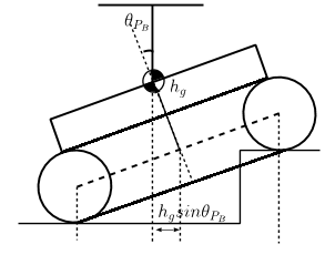
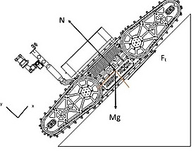
As mentioned in earlier sections, the competition field contains obstacles whose height reaches, at most, the combined height of three stacked pipes, and the robot needs the capability to climb over these obstacles.
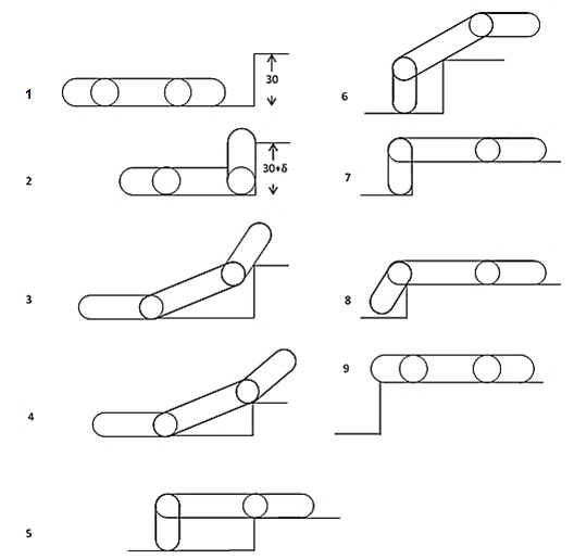
Computing the Mobile Base Robot's Dimensions
In this section, we'll examine the force balance acting on the robot.
Figure 5-4: Schematic view of the robot
Figure 5-5: Force diagram
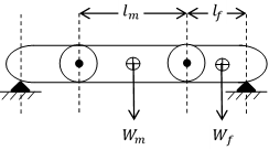
Computing the Forces Acting on the Robot's Arm
Figure 5-6: Schematic view of the robot
Figure 5-7: Schematic view of the robot
Figure 5-8: Schematic view of the robot
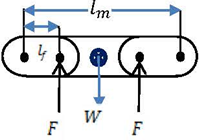
Figure 5-9: Schematic view of the robot
Computing the Power of the Motors Used in the Robot
- The required torque for each motor works out to 23 newton-meters.
Resulted Speed of Flippers = 8 rpm
Computing the Forces Acting on the Robot While Climbing an Inclined Surface
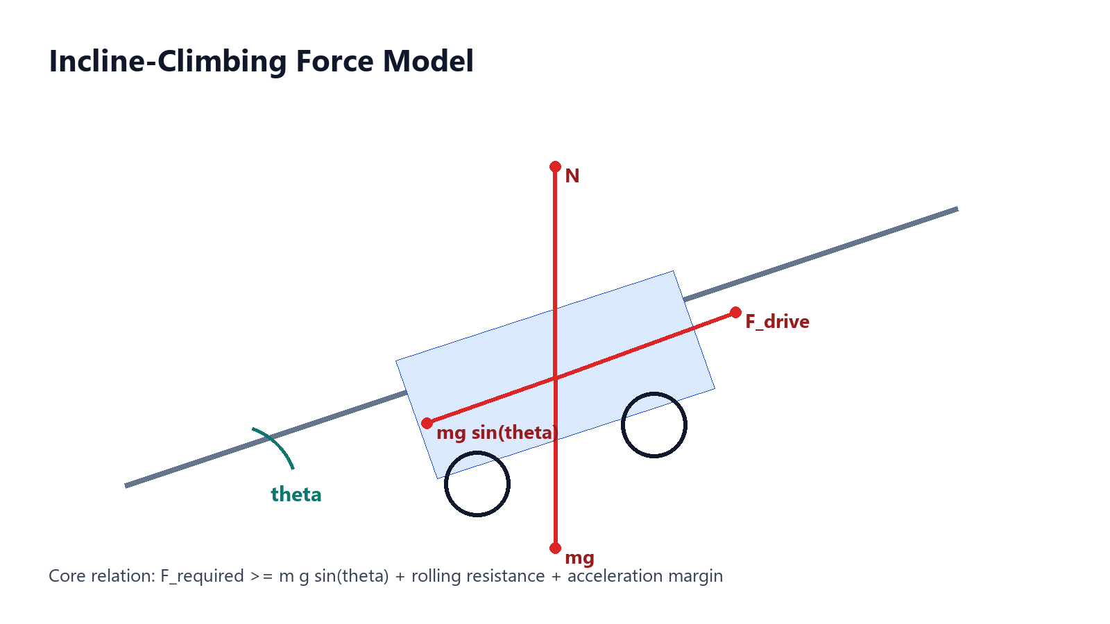
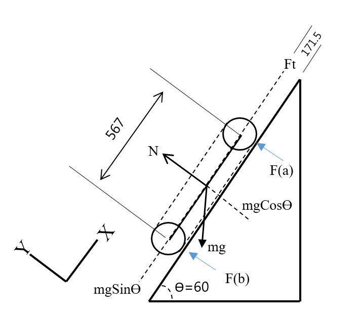
- The required torque for climbing the inclined surface works out to 22.35 newton-meters, so a 25 newton-meter motor is preferred.
Images of the Robot Designed in SolidWorks
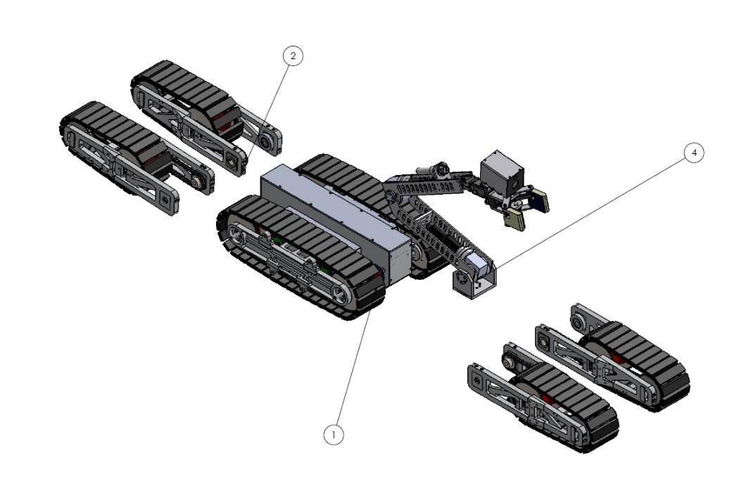
- The Robot's Main Body Section
- The Rear Arm (Flipper) Section
- The Front Arm (Flipper) Section
- 5-Degree-of-Freedom Arm
- Front View of the Robot with Arms Extended
- This robot was calculated and designed based on a tracked-wheel system.
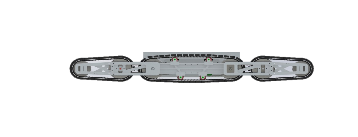
- View of the Robot with Arms Retracted
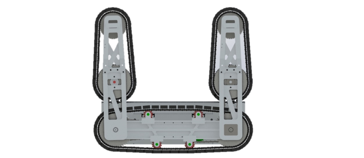
Here, the arms are positioned at 90 degrees.
Figure 5-14: View of the Robot
- Overall View of the Robot
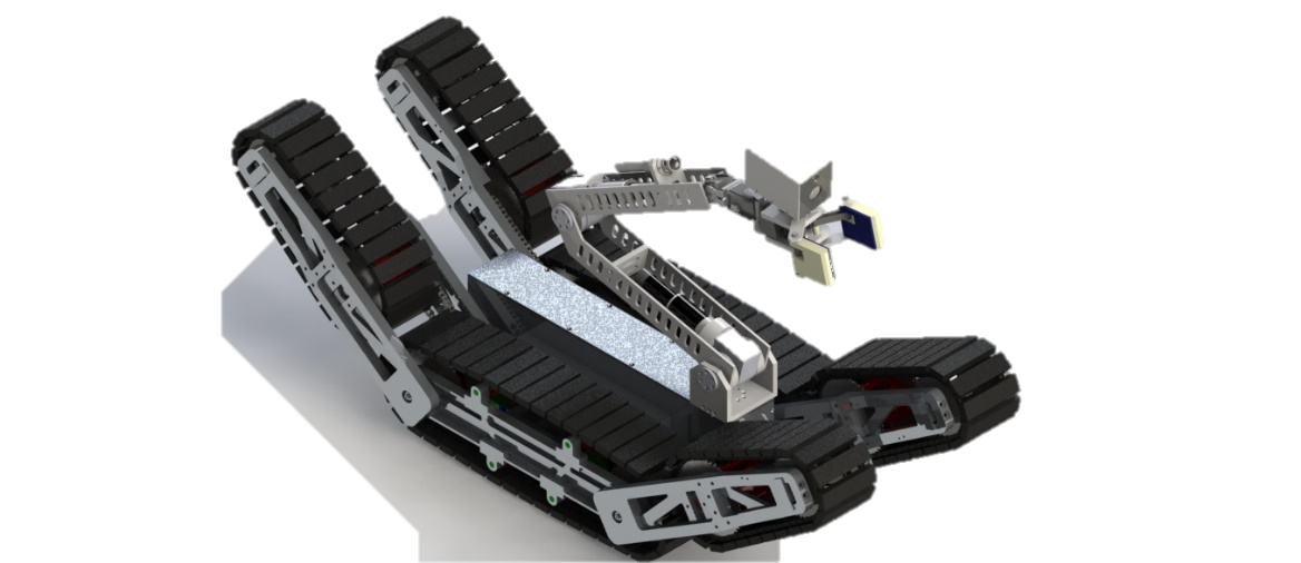
- Interior View of the Robot (Motors, etc.)
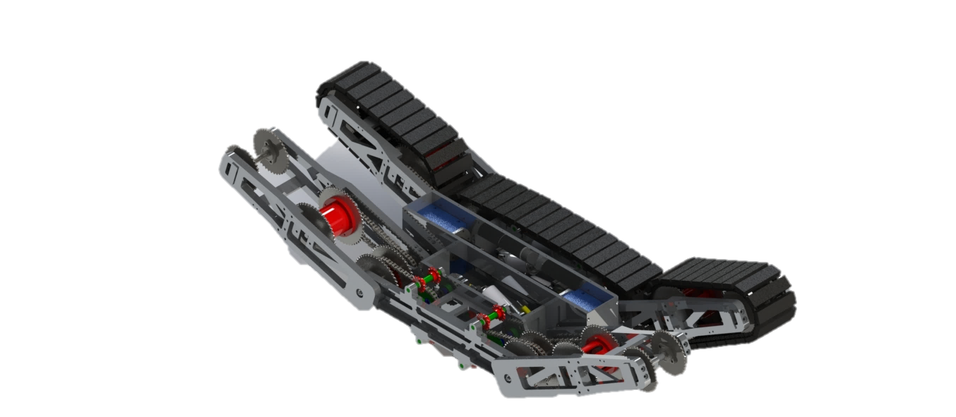
- The motor used in this robot is a German-made Buhler motor.
Designing the Driver Circuit for Controlling the Robot
The Robot's Power Supply Circuit
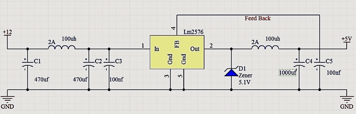
- One of the best options in robotic systems is using off-the-shelf DC-to-DC converters, since they're highly resistant to magnetic and EMI noise and have a very simple driver circuit. But for smaller sections, as mentioned earlier, you can use the circuit shown in Figure 5-15.
Figure 5-15: LM2576 Switching Circuit
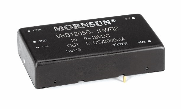
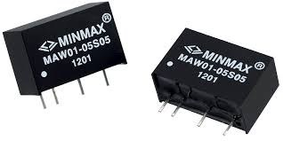
Figure 5-16: DC-DC Switching Circuit
Motor Driver Circuit for DC Drive Systems
To drive low-power DC motors, you can use an L298 or L6203 circuit, and, using H-bridge principles, you can also design a closed control circuit using relays, or MOSFETs and power transistors. But the market also offers plenty of tested, industrial-grade motor drivers - Devantech's products, for example. Take the MD03, a medium-power motor driver that's more capable than many available H-bridges. Ease of use and flexibility are among this driver's standout features. The motor is controlled through pulse-width modulation (PWM), which drives the H-bridge's transistors.
Figure 5-17: L298 Driver Circuit for Low-Power Motors
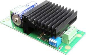
Figure 5-18: Devantech's MD03 Motor Driver
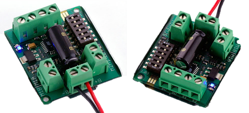
Figure 5-19: Sabertooth High-Power Motor Driver with Dual 25-Amp Outputs
The Robot's Controller Circuit
To coordinate between the various sections and carry out commands issued through the computer, a controller unit is needed to send forward/backward and other commands to the other units. This is where a fast microcontroller plays an important role. You can use an FPGA or an ARM chip here - this section is entirely optional, but we'll introduce a few good controller units below. The RoBoard RB-110 is a powerful, lightweight, portable computer designed specifically for robotics applications. The RB-110's processor, from the Vortex86DX family, is a 32-bit x86 processor that can run at 1000 MHz with 256MB of memory. Various operating systems, such as Windows and Linux, can be installed on this small computer, and using its open-source C++ library, you can make the robot smart through its various interfaces. This board is also a good way to use Microsoft Robotics Studio software to control the robot.
Figure 5-20: Industrial Computer with Enough Ports to Control the Robot
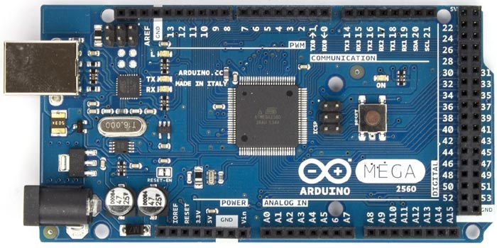
Figure 5-21: Arduino Controller Board
Buying the Parts Needed to Build a Robot
Sourcing the parts needed to build a robot is one of the most important parts of the process, and it usually comes with its share of headaches - the quality of purchased goods, as well as parts availability, has always been a concern for robotics students. This section tries to give a general overview of where to buy the parts needed to build a robot.
Mechanical
Electronics
Online Robotics Store
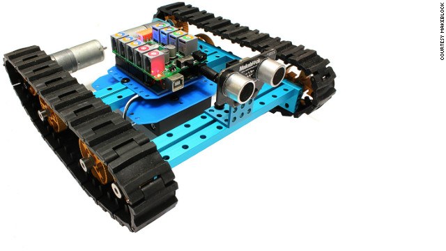
Microcontroller Architectures for Mobile Robots
↑ Table of Contents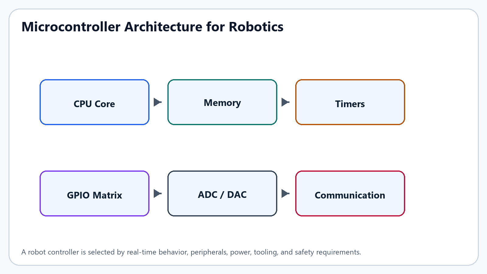
A microcontroller is not chosen only by clock speed. In a mobile robot, the controller must read sensors at predictable intervals, generate motor commands with low jitter, survive electrical noise, recover safely from software faults, and communicate with higher-level autonomy software. The correct architecture is therefore the one whose timing, peripherals, memory, power behavior, and development tools match the robot's mission.
Core Architectural Families
| Architecture | Typical Strength | Robotics Use |
|---|---|---|
| 8-bit MCU | Simple, inexpensive, deterministic for small tasks | Buttons, LEDs, simple sensors, educational subsystems |
| 32-bit ARM Cortex-M | Strong peripheral set, low power, broad tooling | Motor control, sensor hubs, real-time embedded controllers |
| ESP32-class SoC | Wireless connectivity, dual-core variants, rich peripheral matrix | Connected robot controllers, telemetry, edge control, Wi-Fi or BLE links |
| Linux SBC | High compute, vision, ROS 2, AI acceleration through attached hardware | Perception, mapping, planning, user interface, data logging |
| FPGA or real-time co-processor | Very low latency and parallel signal processing | High-speed encoders, custom motor control, hard real-time acquisition |
A robust mobile robot often uses more than one computing layer. The microcontroller handles deterministic control and safety, while a single-board computer or industrial computer handles mapping, planning, perception, and AI. This separation prevents a heavy vision or navigation process from interrupting motor safety behavior.
A simple way to understand the architecture is to imagine a robot as a body with two brains. The small brain is the microcontroller: it reacts quickly, keeps balance, reads encoders, and stops the motors when something is wrong. The large brain is the onboard computer: it looks at camera images, builds maps, thinks about where to go, and talks to the operator. A good robot gives each brain the job it can do best.
Selection Criteria
- Timing: control loops for wheel velocity often run at 50-500 Hz, while encoder capture may need much faster edge counting.
- Peripheral fit: count PWM channels, quadrature encoder inputs, ADC channels, UART, SPI, I2C, CAN, and emergency-stop inputs before selecting the board.
- Electrical robustness: motor current, ground bounce, EMI, and long cables can corrupt signals unless isolation, filtering, and grounding are designed carefully.
- Software maintainability: choose a toolchain that supports version control, repeatable builds, unit tests where practical, and readable driver structure.
- Safety behavior: the controller must define a safe output state for boot, reset, communication loss, watchdog timeout, low battery, and motor-driver faults.
Engineering Decision Rule
Choose the smallest controller that can meet timing and safety requirements with margin. Do not use a large Linux computer for millisecond-level motor protection, and do not force a small microcontroller to run vision, mapping, and AI. The architecture is correct when each computing layer has a clear responsibility and the robot remains safe when any non-safety layer fails.
Modern Embedded Control with ESP32
↑ Table of Contents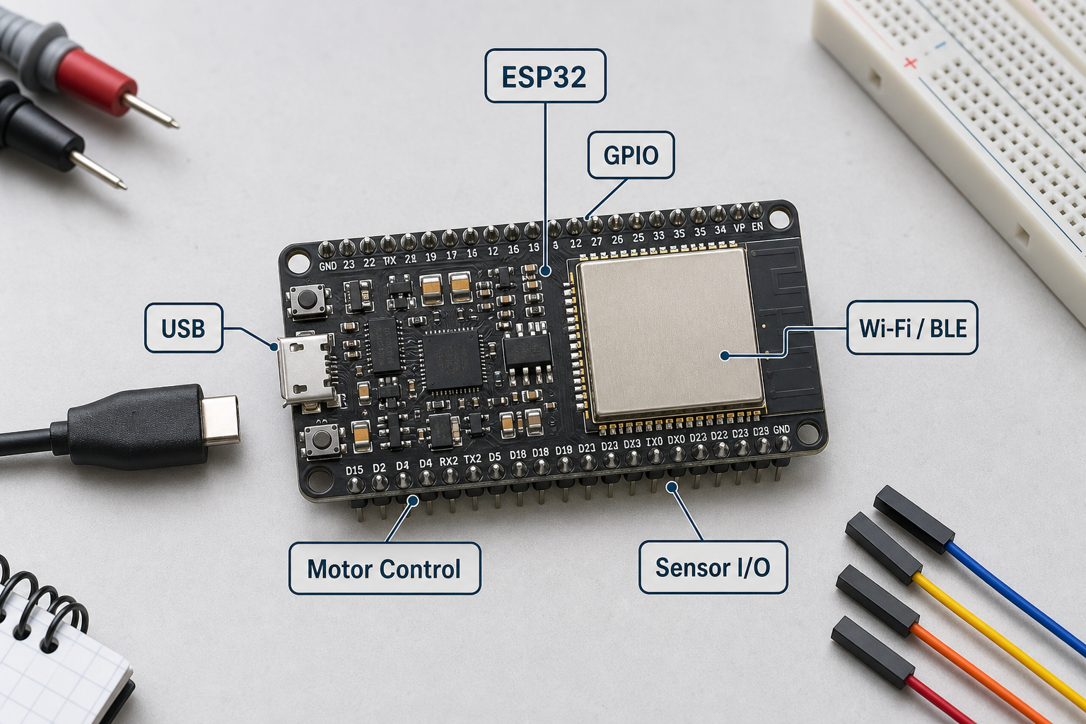
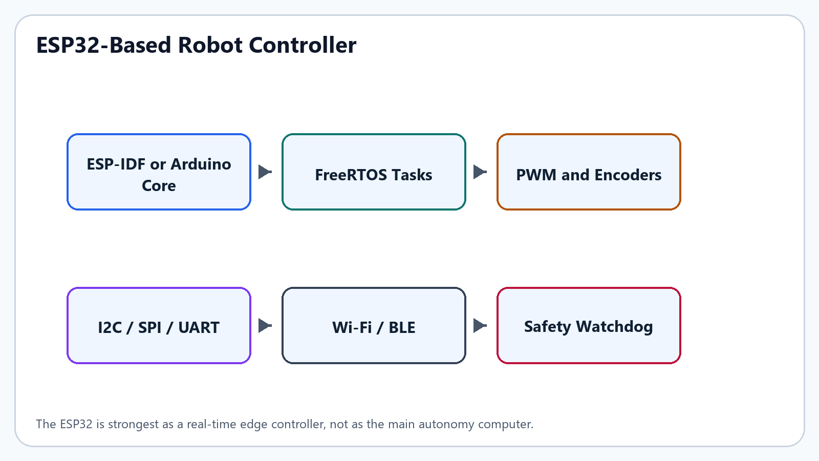
For a contemporary mobile robot, the ESP32 family is a practical replacement for older educational microcontroller workflows. It combines low cost, wireless connectivity, hardware timers, PWM, ADC, serial interfaces, and a mature software ecosystem. In professional designs, the ESP32 is usually best placed as an embedded edge controller that reads encoders and sensors, drives motor controllers, runs safety tasks, and exchanges commands with a higher-level computer.
The official ESP-IDF workflow configures a project, builds it, flashes firmware onto the board, and monitors serial output. Arduino Core and PlatformIO can be useful for teaching and rapid prototypes, while ESP-IDF is preferable when the robot requires clearer task scheduling, lower-level peripheral control, reproducible builds, or production-style firmware organization. Current ESP-IDF documentation describes IDF FreeRTOS as a FreeRTOS implementation modified for ESP targets, including dual-core SMP behavior on supported chips.
Recommended ESP32 Robot Architecture
- One real-time task reads wheel encoders at a fixed period and estimates wheel speed.
- One control task runs the velocity loop and updates PWM or motor-driver commands.
- One communication task handles Wi-Fi, BLE, UART, CAN bridge, or micro-ROS messages.
- One safety task monitors battery voltage, motor-current faults, watchdog state, and emergency stop input.
- Configuration values such as PID gains, wheel radius, encoder counts per revolution, and maximum current are stored as versioned parameters.
Minimal ESP32 Control Example
The following compact example shows the structure of a wheel-speed controller. It is intentionally short; real robots should add encoder interrupt handling, current limiting, watchdog reset, and a safe stop state.
In firmware, the loop period dt must be measured or enforced by a timer. If dt changes without being included in the calculation, the integral and derivative terms become inconsistent and the robot will behave differently at different CPU loads.
ESP32 Training Path
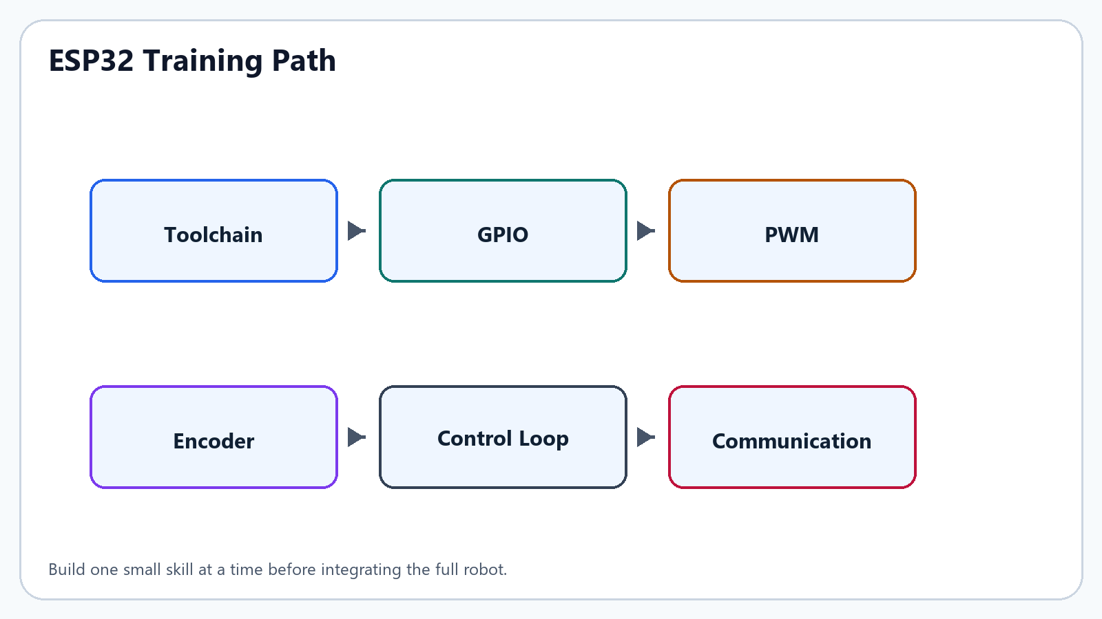
A student should learn ESP32 robotics in small, testable steps. Do not begin by building the whole robot. Begin by proving that the board, toolchain, one output, one input, one motor driver, and one encoder each work independently.
| Lesson | Goal | What the Student Should Prove |
|---|---|---|
| 1. Toolchain | Install ESP-IDF or a supported IDE workflow | A simple example builds, flashes, and prints serial output. |
| 2. GPIO | Read a button and drive an LED or logic output | Input state changes are detected reliably. |
| 3. PWM | Generate a motor command using LEDC or MCPWM | Duty cycle changes motor speed through a driver. |
| 4. Encoder | Count wheel pulses using interrupt or PCNT | Counts increase and decrease with correct direction. |
| 5. Control Loop | Run a fixed-period velocity controller | Measured wheel speed approaches target speed smoothly. |
| 6. Communication | Receive velocity commands from host computer | Timeout stops the robot if commands disappear. |
ESP32 Practical Exercise: One Wheel Velocity Loop
- Mount one motor, one wheel, one motor driver, and one encoder on the bench before installing them in the robot.
- Flash firmware that prints encoder counts every 100 ms. Rotate the wheel by hand and confirm the count changes in the expected direction.
- Add PWM output and test the motor at low duty cycle while the wheel is lifted safely off the ground.
- Compute measured_speed from encoder ticks and sample time.
- Add a proportional controller first. Increase Kp slowly until speed follows the command without violent oscillation.
- Add integral action only after the proportional loop is stable. Limit the integral term so it cannot wind up while the motor is saturated.
ESP32 Wheel-Speed Error
| Symbol | Meaning |
|---|---|
| error | The speed difference the controller tries to remove. |
| target_speed | The desired wheel speed sent by the robot software or test program. |
| measured_speed | The actual wheel speed estimated from encoder ticks. |
If error is positive, the wheel is too slow and the controller should increase motor command. If error is negative, the wheel is too fast and the command should decrease.
Discrete PID Motor Command
| Symbol | Meaning |
|---|---|
| u_k | Motor command at the current sample. It is usually converted to PWM duty cycle. |
| e_k | Current error: target speed minus measured speed. |
| e_{k-1} | Previous error from the last control cycle. |
| dt | Time between control updates in seconds. |
| Kp | Proportional gain. It reacts to present error. |
| Ki | Integral gain. It reacts to error that remains over time. |
| Kd | Derivative gain. It reacts to how quickly the error is changing. |
Start with Kp only. Add Ki when the wheel cannot quite reach the target speed. Add Kd only when measurement noise is controlled, because derivative action amplifies noisy encoder estimates.
Practical ESP32 Design Notes
- Do not assign every task the highest priority. Give motor safety and time-critical sampling priority, and keep logging, networking, and diagnostics lower.
- When Wi-Fi is active, verify ADC pin choices carefully. On classic ESP32 parts, ADC2 has documented restrictions when Wi-Fi is used, so ADC1 pins are often safer for analog robot measurements.
- Use hardware PWM and pulse-counting peripherals where available. Software timing loops are easy to write but fragile under communication load.
- Separate motor power from logic power, use common grounding intentionally, and add protection against reverse polarity, voltage spikes, and brownout reset.
- A communication timeout must stop the robot locally. A wireless robot must never continue driving merely because the host computer stopped sending commands.
ESP32 Peripheral Map for Mobile Robots
| Function | Typical ESP32 Interface | Design Note |
|---|---|---|
| DC motor command | PWM, MCPWM, or LEDC | Use a driver with current capacity above stall current. |
| Wheel encoder | GPIO interrupt or PCNT | Prefer hardware pulse counters when available. |
| IMU | I2C or SPI | SPI is more robust at high sample rates. |
| Range sensor | UART, I2C, CAN bridge, or GPIO | Budget timing jitter before using range data in control. |
| Host computer link | UART, USB serial, Wi-Fi, BLE, or micro-ROS bridge | Keep safety-critical stop logic local to the controller. |
Robot Computers: ESP32, Raspberry Pi, and NVIDIA Jetson
↑ Table of Contents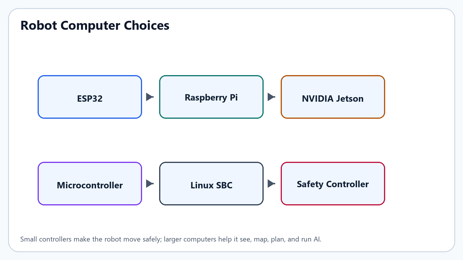
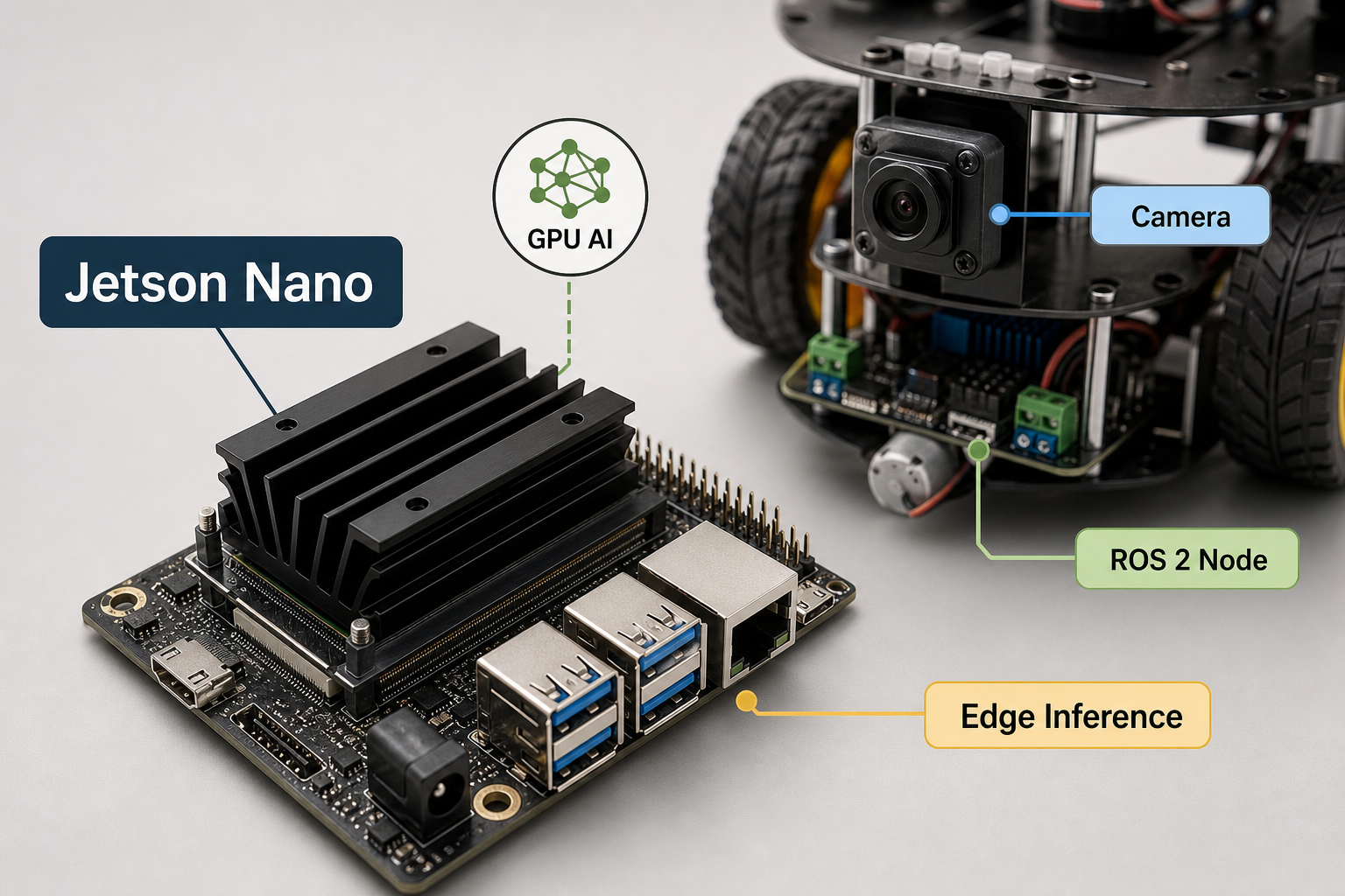
Robotics beginners often ask whether they should use an ESP32, a Raspberry Pi, or an NVIDIA Jetson. The answer is that these boards do different jobs. ESP32 is excellent for direct control and simple wireless communication. Raspberry Pi is a small Linux computer that can run higher-level programs, cameras, logging, dashboards, and light ROS 2 workloads. NVIDIA Jetson is designed for edge AI and robotics workloads that need GPU acceleration, such as deep-learning perception, Isaac ROS packages, and heavier camera pipelines.
| Board Type | Best Job on a Robot | Easy Explanation |
|---|---|---|
| ESP32 | Motor control, encoders, simple sensors, safety stop, Wi-Fi or BLE telemetry | The fast reflexes of the robot. |
| Raspberry Pi 5 | Linux, ROS 2 learning, camera work, data logging, web UI, medium-level autonomy | A small general-purpose computer for thinking and organizing. |
| Raspberry Pi with AI HAT | Local vision AI using a Hailo NPU | A Raspberry Pi with a helper chip that runs neural networks more efficiently. |
| NVIDIA Jetson Orin | GPU-accelerated perception, Isaac ROS, deep learning, multi-camera robots | A stronger onboard AI computer for robots that need to see and understand more. |
| Industrial PC | High-reliability autonomy, fleet robots, harsh environments | A rugged computer when reliability matters more than price. |
How These Computers Work Together
- The ESP32 reads wheel encoders and keeps the motor loop stable even if the main computer is busy.
- The Raspberry Pi or Jetson runs ROS 2 nodes for mapping, camera processing, navigation, logging, and user interfaces.
- The host computer sends desired velocity commands, not raw transistor-level motor signals.
- The ESP32 checks for timeout. If commands stop arriving, it reduces motor output to zero.
- For AI vision, use Raspberry Pi AI HAT or Jetson when the camera workload is too heavy for the CPU alone.
Think of it like a bicycle. The ESP32 is like your hands making tiny steering corrections all the time. The Raspberry Pi or Jetson is like your eyes and planning brain deciding which street to take. If the planning brain gets distracted, the hands still need to keep the bicycle from crashing.
Common Integration Mistakes
- Sending raw PWM commands from the Linux computer instead of sending velocity setpoints to the embedded controller.
- Running camera, mapping, web dashboard, and motor safety on one overloaded processor without a watchdog layer.
- Ignoring boot order: the robot should not move unexpectedly while the host computer is still starting.
- Using Wi-Fi as if it were a deterministic real-time control link. Wireless communication is useful, but safety must be local.
- Choosing Jetson or Raspberry Pi before estimating camera count, frame rate, model size, power budget, and cooling needs.
Odometry for Mobile Robots
↑ Table of Contents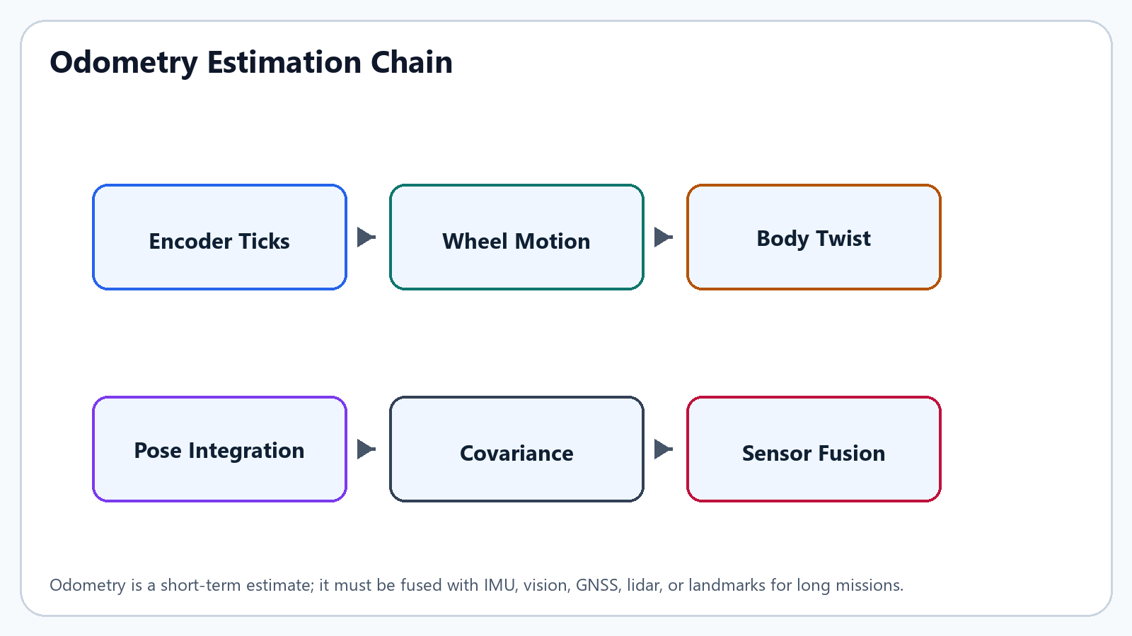
Odometry estimates the robot's pose by integrating measured motion over time. It is essential because it gives the controller a fast local estimate of movement, but it is never perfect. Wheel slip, uneven ground, encoder quantization, tire deformation, backlash, calibration error, and timing jitter accumulate into drift. For this reason, odometry should be treated as a short-term estimate and fused with additional sensors whenever the robot must navigate for long periods.
Differential-Drive Odometry
| Symbol | Meaning |
|---|---|
| Delta s_L | Distance traveled by the left wheel during one sample. |
| Delta s_R | Distance traveled by the right wheel during one sample. |
| r | Wheel radius, measured under the robot's normal load. |
| Delta phi_L | Left wheel rotation angle during the sample, in radians. |
| Delta phi_R | Right wheel rotation angle during the sample, in radians. |
The left and right wheel displacements are obtained from wheel radius r and measured wheel angle changes Delta phi_L and Delta phi_R. If encoders report ticks, the angle increment is Delta phi = 2*pi*Delta ticks / N, where N is encoder counts per wheel revolution after gearbox and quadrature decoding are accounted for.
In plain language: if a wheel turns a little, the robot moves a little. A bigger wheel moves farther for the same rotation. An encoder is like a tiny counter attached to the wheel; it tells the robot how many small steps the wheel has turned.
| Symbol | Meaning |
|---|---|
| Delta s | Forward movement of the robot center during one sample. |
| Delta theta | Change in robot heading during one sample. |
| L | Effective distance between left and right wheel contact lines. |
| Delta s_R - Delta s_L | Difference between right and left wheel travel; this creates turning. |
Delta s is the approximate forward displacement of the robot center, Delta theta is the heading change, and L is the effective wheel separation. The word effective matters: the value that best fits real motion can differ slightly from the mechanical drawing because tires deform and the contact patch is not ideal.
If both wheels move the same distance, the robot goes straight. If the right wheel moves farther than the left wheel, the robot turns left. If the left wheel moves farther than the right wheel, the robot turns right. This is why a tank-like robot can turn without a steering wheel.
| Symbol | Meaning |
|---|---|
| x_k, y_k | Robot position on the map before the update. |
| x_{k+1}, y_{k+1} | Robot position on the map after the update. |
| theta_k | Robot heading before the update. |
| theta_{k+1} | Robot heading after the update. |
| cos, sin | Functions that split forward movement into x and y map directions. |
| wrap | Operation that keeps the angle inside a standard interval, usually -pi to pi. |
The midpoint heading theta_k + Delta theta/2 gives a better small-arc approximation than using only the old heading. The wrap operation keeps the angle inside a chosen interval, usually -pi to pi.
The x and y formulas simply answer this question: after the robot moves forward, where is it now on the floor map? If it faces east, most movement changes x. If it faces north, most movement changes y. The cosine and sine functions are the mathematical way of splitting forward movement into map directions.
Odometry Error and Calibration
- Measure wheel radius under load; unloaded tire diameter can be misleading.
- Estimate effective wheel separation by commanding rotations and comparing measured heading against ground truth.
- Timestamp encoder samples and IMU samples. Unsynchronized data can create apparent drift even when the sensors are good.
- Publish covariance with odometry in ROS 2. Navigation and sensor-fusion systems need uncertainty, not only pose values.
- Use IMU yaw-rate data to improve short-term heading, but do not assume a low-cost IMU eliminates wheel-slip error by itself.
Odometry Debugging Checklist
- Push the robot forward by hand and confirm x changes in the correct direction.
- Rotate the robot in place and confirm yaw changes with the correct sign.
- Drive one meter forward and measure whether the odometry also reports approximately one meter.
- Spin the robot 360 degrees and adjust effective wheel separation if the reported angle is too small or too large.
- Plot odometry and IMU yaw together. If they disagree during straight motion, check wheel diameter, encoder polarity, and frame transforms.
SLAM: Simultaneous Localization and Mapping
↑ Table of ContentsSLAM is the problem of estimating a map and the robot trajectory at the same time. It is central to autonomous mobile robots because the robot often begins without a reliable map, while localization itself requires some representation of the environment. Modern systems solve this circular dependency with probabilistic estimation, scan matching, feature tracking, graph optimization, or combinations of lidar, camera, IMU, wheel odometry, GNSS, and landmarks.
SLAM State Model
| Symbol | Meaning |
|---|---|
| p(...) | Probability distribution; it represents uncertainty, not a single guaranteed answer. |
| x_1:t | Robot pose history from time 1 to time t. |
| m | Map of the environment. |
| z_1:t | Sensor measurements collected over time. |
| u_1:t | Motion inputs or odometry estimates collected over time. |
This compact expression means: estimate the history of robot poses x_1:t and map m given measurements z_1:t and control or odometry inputs u_1:t. It is not a single algorithm; it is the estimation problem that algorithms such as EKF-SLAM, particle-filter SLAM, graph-based SLAM, lidar SLAM, and visual-inertial SLAM attempt to solve.
For a young reader, SLAM can be understood like this: imagine walking in a dark room with a flashlight while drawing a map. You do not know exactly where you are, and you do not know the room shape yet. Every time you see a wall, chair, or door, you improve the map; every time the map improves, you also understand your own position better. SLAM is the robot version of doing both at once.
| Symbol | Meaning |
|---|---|
| x_t | Robot pose at the current time. |
| x_{t-1} | Robot pose at the previous time. |
| u_t | Motion input or odometry measurement. |
| f(...) | Motion model: predicts where the robot moved. |
| z_t | Current sensor measurement. |
| h(...) | Measurement model: predicts what the robot should see. |
| w_t | Motion uncertainty, such as slip or imperfect actuation. |
| v_t | Sensor uncertainty, such as noise, blur, or lidar error. |
The motion model f predicts the next pose from the previous pose and input. The measurement model h predicts what the sensors should observe from a pose and a map. The terms w_t and v_t represent process noise and measurement noise. If those uncertainties are ignored, the map may look precise while the robot's actual position estimate is unreliable.
The first part says, 'Where do we think the robot moved?' The second part says, 'What should the robot see if it is really there?' If prediction and observation disagree, the SLAM system adjusts the estimate. The noise terms remind us that wheels slip and sensors are imperfect.
Choosing a SLAM Approach
| Approach | Best Fit | Main Limitation |
|---|---|---|
| 2D lidar SLAM | Indoor ground robots and structured environments | Can struggle with glass, sparse geometry, and strong vertical structure changes |
| Visual SLAM | Camera-rich platforms and textured environments | Sensitive to lighting, blur, low texture, and calibration |
| Visual-inertial odometry | Small robots, drones, and fast motion | Requires careful camera-IMU timing and calibration |
| Graph-based multi-sensor SLAM | Robots needing loop closure and long missions | More complex compute, tuning, and validation |
- Use loop closure carefully. A false loop closure can damage an otherwise usable map.
- Keep raw logs. SLAM failures are difficult to diagnose if only the final map is saved.
- Evaluate maps with repeated runs, not a single successful demonstration.
- For safety-critical navigation, pair SLAM with obstacle detection and local stop behavior that does not depend on a perfect map.
What Makes a Good Map?
A good SLAM map is not the prettiest image; it is the map that helps the robot localize and navigate repeatably. Straight walls should remain straight, loop closures should not bend corridors unnaturally, doorways should remain passable, and obstacles should appear where the robot's sensors can consistently observe them. A map that looks clean after one run but fails on the next run is not an engineering result yet.
ROS 2 Architecture for Mobile Robots
↑ Table of Contents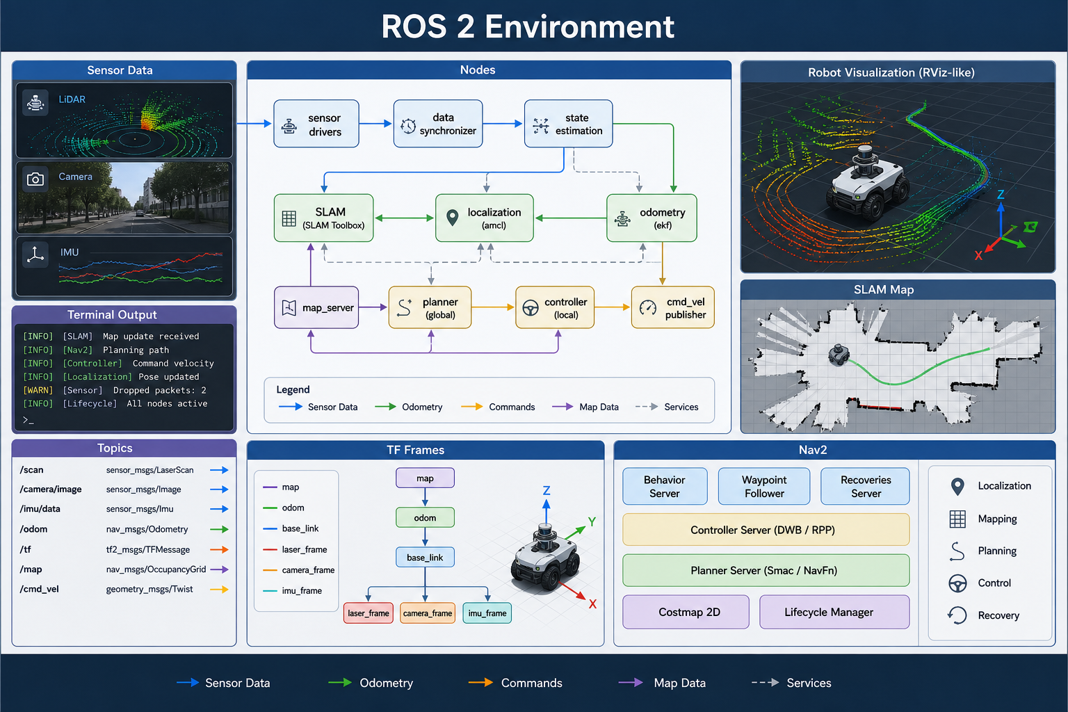
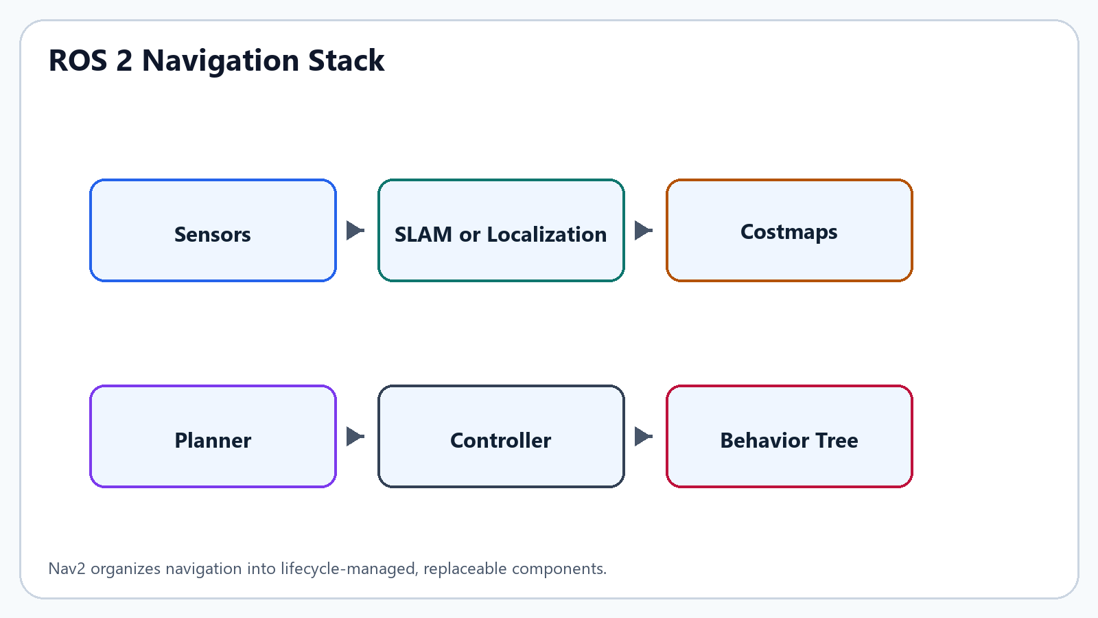
ROS 2 is the modern middleware foundation for many mobile robots because it supports modular nodes, typed messages, discovery, parameters, launch files, visualization, logging, and distributed computation. In a clean architecture, the embedded controller maintains deterministic motor and safety behavior, while ROS 2 handles perception, mapping, planning, operator tools, and data recording.
ROS 2 decomposes a robot into nodes. Nodes exchange continuous data through topics, request quick operations through services, and execute long-running goals through actions. Navigation is a natural action use case: the robot receives a goal, reports feedback while moving, and eventually returns success, failure, or cancellation.
A simple classroom analogy helps: ROS 2 is like a school where every student has one job. One student watches the camera, one listens to the lidar, one estimates position, one plans the route, and one sends speed commands. Topics are like notice boards where students continuously post information. Services are quick questions. Actions are bigger assignments that take time, such as 'go to the door and tell me when you arrive.'
ROS 2 Communication Patterns
| Pattern | Use It For | Mobile Robot Example |
|---|---|---|
| Topic | Streaming data with many possible publishers/subscribers | Laser scans, camera images, odometry, velocity commands |
| Service | Short request-response operations | Reset odometry, save a map, query controller mode |
| Action | Long-running tasks with feedback and cancellation | Navigate to pose, dock, inspect a waypoint |
| Parameter | Runtime configuration | PID gains, frame names, speed limits, sensor rates |
Frames and Transforms
A professional ROS 2 robot must define coordinate frames clearly. The common chain is map -> odom -> base_link, with additional frames for lidar, camera, IMU, wheels, and manipulators. The map frame is globally consistent when localization or SLAM is working. The odom frame is locally smooth but drifts over time. The base_link frame is fixed to the robot body. Confusing these frames is one of the most common causes of navigation failure.
Another simple explanation: base_link is the robot's belly button. odom is where the robot thinks it has moved since it started rolling. map is the larger world map. Sensors such as cameras and lidars have their own small coordinate frames because they are mounted in different places on the robot.
Nav2 and the Autonomy Stack
Nav2 is a production-grade navigation framework built on ROS 2. It organizes navigation around localization or SLAM, costmaps, path planning, trajectory control, recovery behaviors, lifecycle-managed nodes, and behavior trees. This structure lets teams replace one component without rewriting the entire autonomy stack.
- The global planner computes a path through the map or global costmap.
- The local controller converts the path into feasible velocity commands while reacting to nearby obstacles.
- Costmaps represent free space, inflated obstacles, unknown regions, and dynamic hazards.
- Behavior trees coordinate navigation, recovery, replanning, waiting, docking, and cancellation behavior.
- Lifecycle nodes make startup, configuration, activation, deactivation, and shutdown more explicit than ad-hoc launch order.
A Practical ROS 2 Node Layout
| Node | Responsibility | Typical Output |
|---|---|---|
| base_controller_bridge | Connects ROS 2 velocity commands to the embedded controller | cmd_vel handling, wheel feedback |
| robot_state_publisher | Publishes fixed and moving transforms from the robot model | tf tree |
| odometry_node | Publishes local pose estimate from encoders and IMU | odom and odom -> base_link |
| sensor_driver_nodes | Publish camera, lidar, IMU, or range data | sensor topics |
| localization_or_slam | Estimates pose in a map or builds the map | map -> odom and occupancy map |
| nav2_stack | Plans and controls navigation behavior | paths, velocity commands, action feedback |
This separation gives the student a powerful debugging advantage. If the robot does not move, inspect the bridge and embedded controller. If it moves but the map drifts, inspect odometry and sensor timing. If the map is good but navigation fails, inspect costmaps, transforms, planner settings, and controller limits.
ROS 2 Training Path
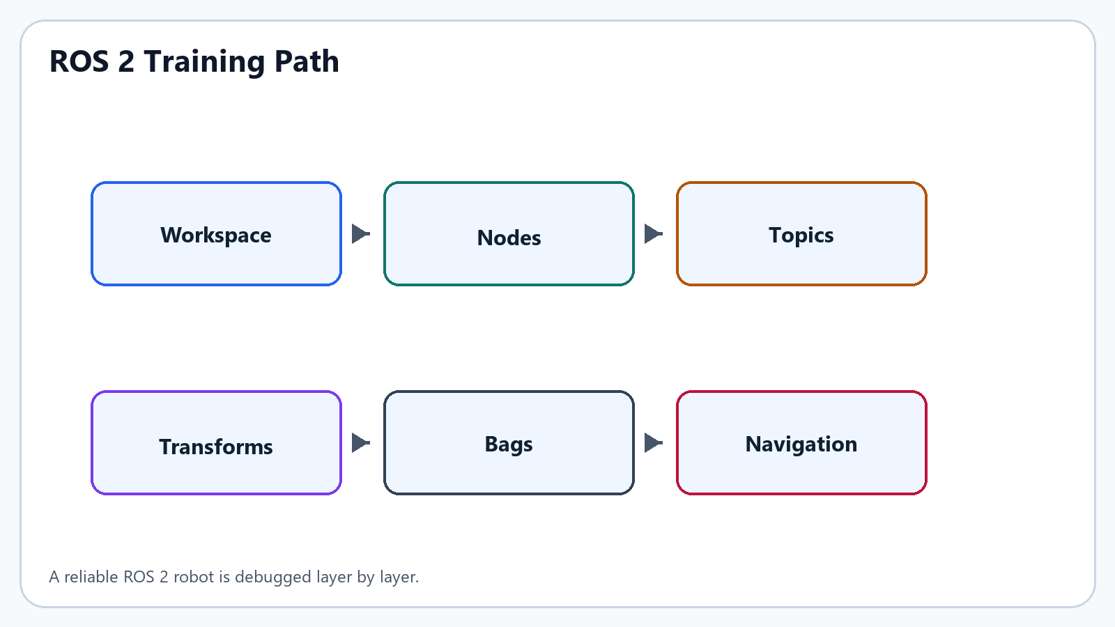
ROS 2 should be learned as a set of small communication skills before it is used for full autonomy. A student who can inspect topics, read transforms, launch nodes, and record data will debug robots much faster than a student who only knows how to start a large launch file.
| Lesson | Skill | Command or Tool |
|---|---|---|
| 1. Workspace | Create and build packages | colcon build |
| 2. Environment | Load the workspace overlay | source install/setup.bash |
| 3. Nodes | List running programs | ros2 node list |
| 4. Topics | Inspect streaming data | ros2 topic list, ros2 topic echo |
| 5. Services | Call request-response functions | ros2 service list, ros2 service call |
| 6. Actions | Send long-running goals | ros2 action list, ros2 action send_goal |
| 7. Launch | Start a multi-node system | ros2 launch |
| 8. Bags | Record evidence for debugging | ros2 bag record |
ROS 2 Practical Exercise: From Teleoperation to Navigation
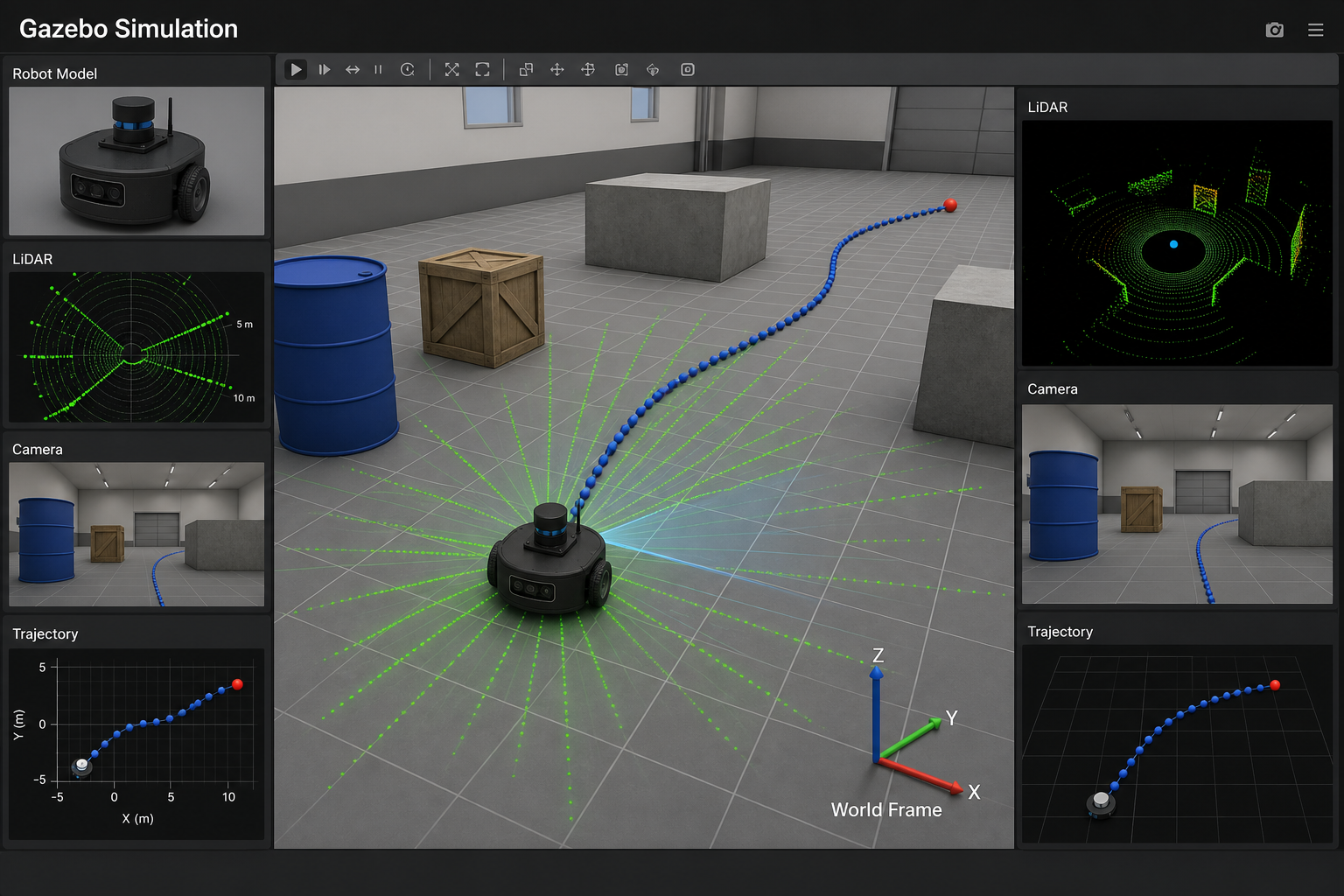
- First, run a simulation or a safe wheeled base with the wheels lifted. Confirm that cmd_vel commands reach the base controller.
- Publish odometry and confirm the odom frame moves smoothly when the wheels turn.
- Add robot_state_publisher and verify that base_link, wheel, sensor, camera, and lidar frames appear in the transform tree.
- Add a lidar or depth camera and inspect the raw sensor topic before using SLAM.
- Run SLAM or localization and confirm that map -> odom changes slowly while odom -> base_link remains smooth.
- Only after those layers work should Nav2 be started for autonomous navigation.
The correct mindset is layer-by-layer evidence. If navigation fails, do not immediately tune Nav2. First prove that motor commands, odometry, transforms, sensor data, map quality, and costmaps are each correct.
Artificial Intelligence in Mobile Robotics
↑ Table of Contents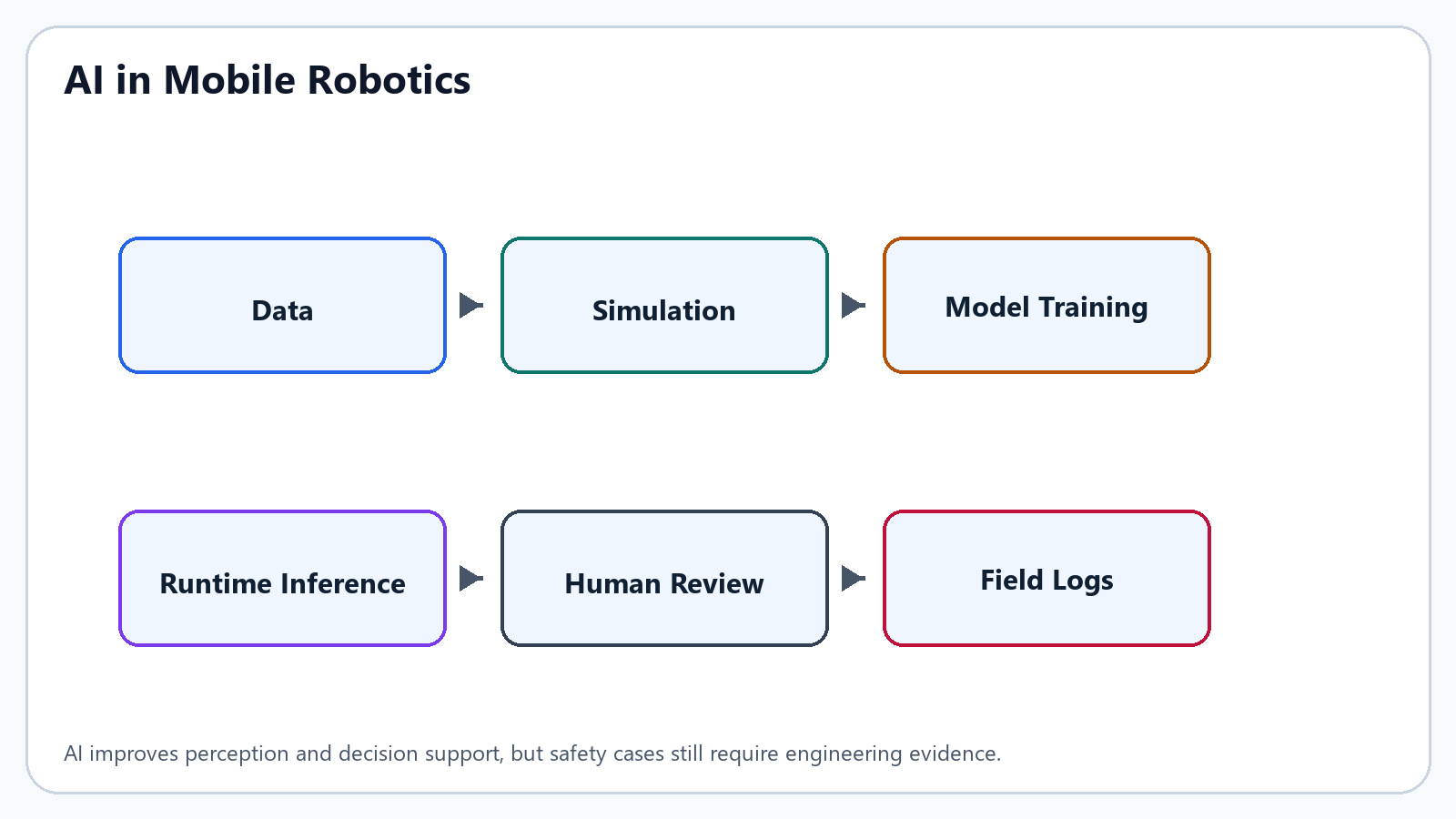
AI should be treated as an engineering tool, not as magic. In mobile robotics it is strongest in perception, semantic understanding, anomaly detection, simulation-assisted design, fleet analytics, and operator decision support. A learning system can detect people, segment drivable terrain, classify objects, predict traversability, or assist with inspection reports, but safety-critical motion still needs explicit limits, monitoring, and validation.
A practical AI workflow begins with data definition: what sensor data are collected, under what lighting, terrain, speed, weather, and battery conditions, and what failure cases matter. The next steps are annotation, training, simulation, hardware-in-the-loop testing, field validation, and continuous monitoring. Models must be versioned just like mechanical drawings and firmware.
Responsible Use of AI
- Use AI to propose designs, generate test cases, summarize logs, and improve perception, but verify claims with measurement.
- Keep a non-AI safety layer for emergency stop, maximum speed, current limits, obstacle stop distance, and watchdog behavior.
- Record the operating design domain: terrain, payload, temperature, slope, lighting, and communication assumptions.
- Measure false positives, false negatives, latency, and robustness before relying on AI output in navigation.
AI Engineering Rule
Use AI where uncertainty is natural, such as recognizing objects, classifying terrain, or summarizing logs. Use deterministic engineering where the robot must obey hard limits, such as emergency stop, maximum speed, motor current, battery cutoff, and collision prevention. A safe robot can benefit from AI, but it should not require a neural network to remember basic safety rules.
Control Systems Made Clear
↑ Table of ContentsControl is the discipline of making a robot do what we intend despite friction, slope, payload changes, battery voltage drop, sensor noise, and imperfect mechanics. A controller is not simply a piece of code; it is the decision rule that converts error into action.
Open-Loop and Closed-Loop Control
In open-loop control, the robot sends a command without checking the result. For example, it may apply 40 percent PWM to a motor and assume the wheel speed is correct. This is simple, but the same command gives different speed when the battery is full, when the robot climbs a slope, or when a wheel touches thick carpet.
In closed-loop control, the robot measures what actually happened and corrects the command. For wheel speed, the encoder measures real speed. The controller compares desired speed with measured speed. The difference is the error. The controller then changes the motor command to reduce that error.
Control Loop Vocabulary
| Term | Meaning | Robot Example |
|---|---|---|
| Reference | What we want | Target wheel speed = 1.0 m/s |
| Measurement | What the sensor reports | Encoder speed = 0.8 m/s |
| Error | Reference minus measurement | 0.2 m/s too slow |
| Controller | Rule that converts error into action | Increase PWM |
| Actuator | Hardware that applies action | Motor and motor driver |
| Plant | The physical system being controlled | Wheel, gearbox, track, chassis |
| Disturbance | Something that changes behavior unexpectedly | Slope, payload, collision, low battery |
Basic Feedback Error
| Symbol | Meaning |
|---|---|
| e(t) | Error at time t. |
| r(t) | Reference or desired value at time t. |
| y(t) | Measured output at time t. |
If the desired speed is 1.0 m/s and the measured speed is 0.8 m/s, the error is 0.2 m/s. The controller's job is to make this error approach zero without oscillation or unsafe motion.
PID Controller
| Symbol | Meaning |
|---|---|
| u(t) | Controller output, such as motor command or steering command. |
| e(t) | Current error. |
| Kp | Proportional gain; reacts to error now. |
| Ki | Integral gain; reacts to error that remains over time. |
| Kd | Derivative gain; reacts to how quickly error is changing. |
| integral(e(t)) | Accumulated error over time. |
| de(t)/dt | Rate of change of error. |
The proportional term pushes immediately. The integral term removes small persistent error. The derivative term adds damping, but it must be filtered because noisy measurements can make derivative control unstable.
How to Tune a Controller Safely
- Start with the robot lifted or restrained so a bad gain cannot cause a crash.
- Use proportional control first. Increase Kp until the response is quick but not violently oscillatory.
- Add Ki only if the system reaches a steady speed below the target. Keep an anti-windup limit on the integral term.
- Add Kd only when the measurement is clean enough. Derivative control on noisy data creates sharp command spikes.
- Test at low speed, then high speed, then with payload, then on slope. A controller tuned on a bench may fail on the floor.
Control Mistakes That Damage Robots
- Ignoring actuator saturation. If the motor command is already at maximum, more integral action cannot create more voltage; it only creates windup.
- Using a slow loop for a fast system. If the controller reacts too late, the robot oscillates or overshoots.
- Filtering too much. A heavily filtered signal looks smooth but may arrive too late for stable control.
- Trusting one test. A controller must be tested with low battery, full payload, slope, different floor material, and abrupt stop commands.
Updated Engineering Formula Reference
↑ Table of ContentsThe formulas below are useful first-order models for mobile robot design. They should be used with measured coefficients and an explicit safety factor. A formula is not a decoration in an engineering book; it is a compact way to describe cause and effect.
How to Read a Formula
Read every formula in three passes. First, identify what the formula is trying to find. Second, identify which physical quantities make the result larger or smaller. Third, ask how each quantity will be measured on the real robot. This habit turns mathematics from something abstract into a design tool.
- If mass appears in a formula, a heavier robot usually demands more force, torque, power, or braking distance.
- If wheel radius appears, remember that larger wheels travel farther per rotation but usually demand more torque.
- If velocity appears squared, speed becomes dangerous quickly; doubling speed can more than double the required stopping space.
- If efficiency appears in the denominator, losses force the battery to provide more power than the wheels deliver.
Differential-Drive Forward Velocity
| Symbol | Meaning |
|---|---|
| v | Forward velocity of the robot center. |
| r | Wheel radius. |
| omega_R | Angular velocity of the right wheel. |
| omega_L | Angular velocity of the left wheel. |
| (omega_R + omega_L)/2 | Average wheel angular velocity. |
Plain-language explanation: average the left and right wheel speeds, then multiply by the wheel radius. If both wheels spin faster, the robot goes faster. If one wheel is slow, the average speed drops.
Differential-Drive Turning Rate
| Symbol | Meaning |
|---|---|
| omega | Yaw rate of the robot; how fast it turns. |
| r | Wheel radius. |
| omega_R - omega_L | Difference between right and left wheel angular velocity. |
| L | Effective distance between the left and right wheel contact lines. |
Plain-language explanation: turning comes from the difference between the wheels. If both sides move equally, there is no turn. If one side moves more, the robot rotates toward the slower side.
Required Wheel Torque on a Slope
| Symbol | Meaning |
|---|---|
| T_wheel | Minimum torque required at each driven wheel. |
| m | Total robot mass. |
| a | Desired forward acceleration. |
| g | Gravitational acceleration, approximately 9.81 m/s^2. |
| theta | Slope angle. |
| C_rr | Rolling-resistance coefficient. |
| r | Wheel radius. |
| n | Number of driven wheels sharing the load. |
Plain-language explanation: the motor must push three things at once: acceleration, the hill pulling the robot backward, and rolling resistance. A heavier robot, a steeper hill, or a larger wheel all require more torque.
Mechanical and Electrical Power
| Symbol | Meaning |
|---|---|
| P_mech | Mechanical power delivered to motion. |
| P_elec | Electrical power drawn from the battery or supply. |
| F | Driving force at the ground. |
| v | Robot velocity. |
| eta | Efficiency of the motor, gearbox, and drivetrain. It is always less than 1. |
Plain-language explanation: pushing hard while moving fast needs more power than pushing gently or moving slowly. Because motors and gears waste some energy as heat, the battery must provide more power than the wheels actually deliver.
Stopping Distance
| Symbol | Meaning |
|---|---|
| d_stop | Total distance needed to stop. |
| v | Robot speed before braking begins. |
| t_latency | Delay between detecting a hazard and braking actually starting. |
| a_brake | Braking deceleration magnitude. |
| v*t_latency | Distance traveled during reaction and computation delay. |
| v^2/(2*a_brake) | Distance traveled while physically braking. |
Plain-language explanation: a robot does not stop the instant it sees an obstacle. First it needs a short thinking time, then it needs space to brake. Doubling speed can make braking distance much larger.
Continuous PID Controller
| Symbol | Meaning |
|---|---|
| u(t) | Controller output. |
| e(t) | Current error. |
| Kp | Proportional gain. |
| Ki | Integral gain. |
| Kd | Derivative gain. |
| integral(e(t)) | Accumulated error. |
| de(t)/dt | Rate of change of error. |
Plain-language explanation: P reacts to the error right now, I remembers old error that has not gone away, and D looks at how fast the error is changing. Together they help the robot correct motion smoothly instead of shaking or drifting.
System Verification and Publishing-Grade Design Workflow
↑ Table of Contents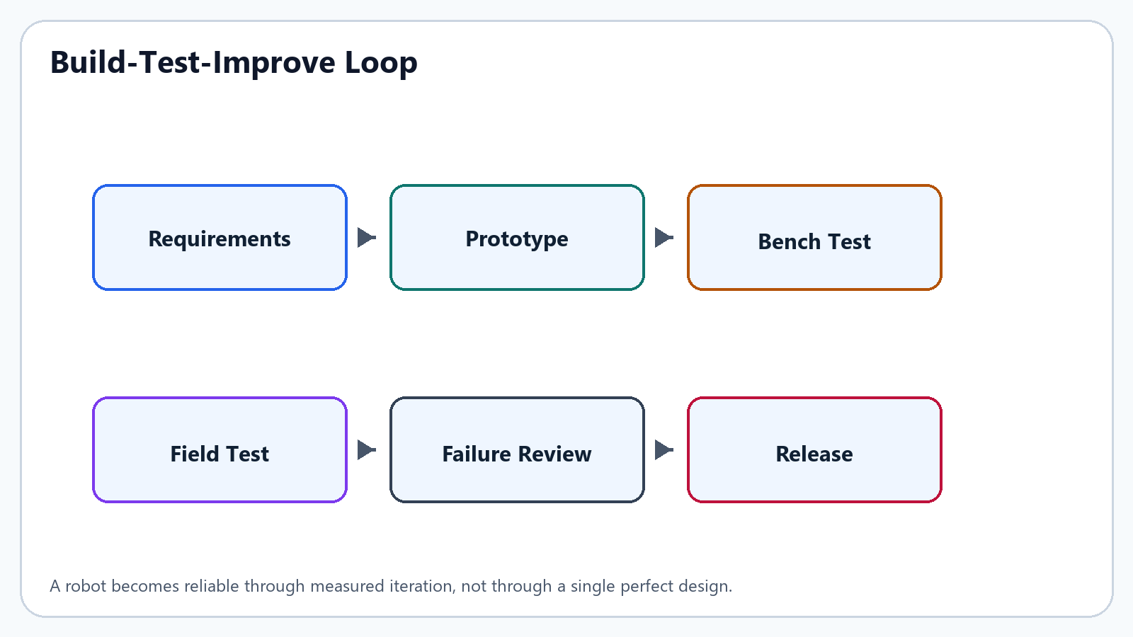
A publishable robotics design is not merely a collection of parts. It is a documented argument that the robot can perform its mission within known limits. The design file should state requirements, assumptions, calculations, interface definitions, failure modes, test procedures, and acceptance criteria.
- Requirements define payload, speed, slope, run time, terrain, sensing range, autonomy level, and safety limits.
- Architecture assigns responsibilities to chassis, drivetrain, power system, embedded controller, autonomy computer, sensors, and software.
- Calculations estimate forces, torque, power, battery capacity, thermal load, and stability margins.
- Prototype tests measure actual current, speed, stopping distance, traction, temperature, localization drift, and communication reliability.
- Failure review converts broken belts, loose fasteners, noisy encoders, unstable control, and software crashes into design improvements.
References and Further Study
↑ Table of Contents- Espressif Systems. ESP-IDF Programming Guide for ESP32, stable documentation.
- Open Robotics. ROS 2 documentation and tutorials.
- Open Navigation LLC. Nav2 documentation and navigation concepts.
- NVIDIA Isaac ROS documentation for accelerated ROS 2 robotics packages and AI models.
- Siciliano, B., Sciavicco, L., Villani, L., and Oriolo, G. Robotics: Modelling, Planning and Control.
- Thrun, S., Burgard, W., and Fox, D. Probabilistic Robotics.